Julia for scientists: the shortest intro
Menu
15:15 Presentation
15:30 Installation
15:40 Live coding
Why would I need another programming language? 🤨
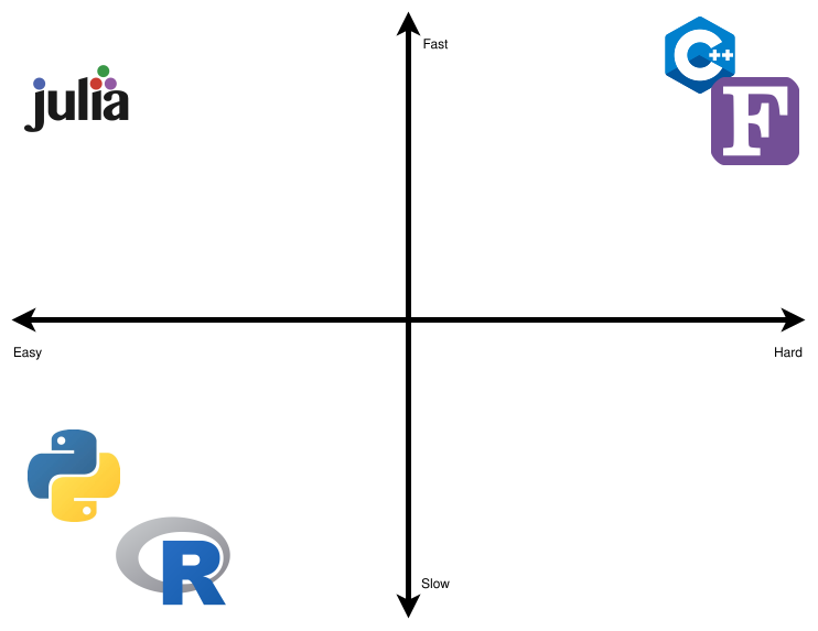
“The two language problem”
- High-level languages (Python, R) are slow because they are interpreted
- Here “interpreted” means the program is not compiled into machine code
- They are executed by a virtual machine that is not specific to a given processor
.gif)
Source geeksforgeeks.org
What are the options for a busy scientist?
- You can either rewrite your code in C, Fortran etc (see you in two years!)
- Or tinker with (pre-)compiling parts of your code:
- Speeding up Python (Cython, Numba) is not too far from learning a new language

Source: scientificcoder.com
- LLVM is a compiler that “translates” your code into byte code. That’s intermediate code, not tied to a specific processor
- In Python, translating to LLVM is not native. It’s optional, e.g. using Numba - it works only for some libraries

Source: scientificcoder.com
- Julia compiles directly to LLVM, all of the code
- Interactive AND compiled
In R you get exposed to the “two-language” problem quickly if you want to look at internals in some statistical packages. Whenever you try to get to how things are actually done and you want to open the “black box”, you’ll find yourself in a world with RCpp and C++ code. […] One of the things that convinced me to give Julia a try was opening the
GLM.jlcode and seeing Julia code inside and being able to follow how data was analyzed, almost step by step, so I could check all the intermediate steps of my calculation.
alejandromerchan on discourse.julialang.org

Source: Julia Data Science
Mathematical notation
\[ g(g_m, I_0, I_k, k, w) = g_m \times \tanh\left(\frac{I_k \exp^{-wk}}{I_k}\right) \]
Julia:
Mathematical notation
#Parameters
ω = 1

#Initial Conditions
x₀ = [0.0]
dx₀ = [π / 2]
tspan = (0.0, 2π)

ϕ = atan((dx₀[1] / ω) / x₀[1])
A = √(x₀[1]^2 + dx₀[1]^2)

#Define the problem
function harmonicoscillator(ddu, du, u, ω, t)
    ddu .= -ω^2 * u
end
Source: DifferentialEquations.jl
Reproducibility
Julia projects are defined using the Project.toml file and optionally Manifest.toml.
If the project contains a manifest, this will install the packages in the same state that is given by that manifest. Otherwise, it will resolve the latest versions of the dependencies compatible with the project.
Substantial backwards compatibility: no need for a completely new install of dependencies for each project.
Multiple dispatch
The same function performs different things depending on the type of the argument.
For example, the gamma function reduces to the factorial function:
\[ \Gamma(n) = (n - 1)! \]
How can I use Julia?
- Julia is Open Source. You can download it at julialang.org and contribute to it
- You can run Julia REPL in the terminal (type
juliaand go!) - You can use a notebook. Ju in Jupyter stands for Julia
- Julia has its own notebook too: Pluto
- Quarto supports Julia
- In this demo we will use Visual Studio Code with Julia Extension. You still need to install Julia!