library(paleobioDB)
library(dplyr)Global plant diversity (R)
In this exercise we like to explore the diversity of the major groups of vascular plants through time. An early attempt at describing it has been made by the super-prolific giant of (paleo)botany, Karl Niklas. You will hear about him in this course again.
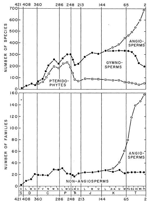
We are asking the question if the data in PBDB is complete enough to obtain the same overall trend. Here we will ignore the early vascular plants and focus on Pteridophytes, Gymnosperms and Angiosperms.
Before you start
Make a new folder for files related to this practical. In R Studio, choose File and New project.... Place the project in the existing folder which you have just created. Whenever you re-open this project, the paths to files will be automatically set.
Objectives
After this practical, you will be able to:
paleobiology skills
Create a diversity (richness) plot for a given taxon
Explain the limitations of fossil data in calculating past diversity
Assess how factors such as sampling effort, taxonomic and temporal resolution affect diversity analyses
data skills
read in functions and apply them to new datasets
present several variables in one plot
Analysing Pteridophyta
In this practical, you will analyse Pteridophyta, Pinophyta and Magnoliophyta. The examples below will guide you through the analysis for Pteridophyta. Afterwards, you will do the same analysis for the other two divisions.
You will need these two libraries installed:
Downloading data from the Paleobiology Database
You can download datasets using the web interface or by sending a direct query to the server using the database’s API. The latter you can do using a script, this way you don’t need to remember what to click. There are ready-made functions which make it easy to download data directly from your script. In the first example, you will use the function pbdb_occurrences from the package paleobioDB by Varela et al. (2015). You need to install this package first.
Pteridophyta <- pbdb_occurrences(
  base_name = "Pteridophyta",
  show = c("coords", "classext"),
  vocab = "pbdb",
  limit = "all"
)
Take a look at the data you have downloaded. What are the rows? Where is the age of each fossil? Where was it found?
1. Genus richness through time
Make a graph showing the genus richness of Pteridophyta over time.
pbdb_richness(Pteridophyta,
              rank = "genus",
              temporal_extent = c(0, 540),
              res = 20)
What happens if you change the parameter res (temporal resolution)? How do you decide which resolution is the best?
Make the same plot but for all three groups: Pteridophyta, Pinophyta and Magnoliophyta.
But the plot made by the paleobioDB package doesn’t allow plotting several groups on the same plot. What now? You can exploit the fact that the function pbdb_richness returns not only a plot, but a dataframe of richness per bin. You can save this dataframe into an object, here called Pteri_rich, and use it to add the remaining two groups to the plot using standard R plotting tools.
Pteri_rich <- pbdb_richness(Pteridophyta,
              rank = "genus",
              temporal_extent = c(0, 540),
              res = 20,
do_plot = F)barplot(names.arg = Pteri_rich$temporal_intervals,
height = Pteri_rich$richness)Try to add the other groups on your own. You can use the parameter add of the barplot function or make a grouped barplot.
2. How to deal with records at different taxonomic levels?
A lot of the time fossils cannot be identified to the species level. Also the concept of species in some groups is not clear. So many analyses rely on the genus level.
Look into the dataframe with the occurrences. Some are observations at the species level, some at the genus level. If you want to analyze richness at the genus level, you have to somehow include also those occurrences which had been made at the species level and discard the species name. E.g. one of the occurrences is Metaclepsydropsis duplex. You still want to count it, but as Metaclepsydropsis. And you still have to consider that some occurrences are of different taxonomic ranks!
This code will show you what taxonomic ranks are present in the dataset:
Pteridophyta$accepted_rank <- as.factor(Pteridophyta$accepted_rank)
levels(Pteridophyta$accepted_rank)
For the rest of the practical you only need records that are at least at the genus level (so species, subgenus and subspecies are ok). You can remove the remaining occurrences. Observe how the dimensions of the dataframe change.
Pteridophyta <- Pteridophyta[Pteridophyta$accepted_rank %in% c("genus", "species", "subspecies","subgenus"),]Now you can extract genus names from those names which also contain species and subspecies. You will need this again so it will be handy to have a function for it. This function takes all rows where the rank is different than genus and extracts the first word of the name.
species_to_genera <- function(df) {
  df$genus_name <- ifelse(
    df$accepted_rank != "genus",
    gsub(" .*", "", df$accepted_name),
    df$accepted_name
  )
  return(df)
}
Now that the function is in memory, you can use it by applying it to the dataset:
Pteridophyta <- species_to_genera(Pteridophyta)So now your analysis will use all the available records which include information about the genus.
3. How precisely do we know the age of a fossil occurrence?
To understand the nature of occurrence data, check in the dataframe how age information is provided. Which variables contain it? What is the average, minimal and maximal time span across the occurrences? In other words, how precise is the age information for each occurrence?
calculate_duration <- function(df, max_ma, min_ma, occ_duration) {
  df[[occ_duration]] <- df[[max_ma]] - df[[min_ma]]
  return(df)
}
Apply the function to your dataset:
Pteridophyta <- calculate_duration(Pteridophyta, "max_ma", "min_ma", "occ_duration")The last column in the dataframe, occ_duration is now the time span assigned to the occurrence, in My.
avg_span <- mean(Pteridophyta$occ_duration)
hist(Pteridophyta$occ_duration,
     xlab = "Occurrence time span [My]",
     main = "Distribution of time spans of pteridophyte occurrences")
abline(v = avg_span,
       col = "red")
What is the average time span of an occurrence in the dataset? Does it mean the fossil lived for so long? Why are some durations so extremely long, i.e. having very low precision? If you were to cull the dataset to eliminate the most imprecisely dated occurrences, what precision would you accept as good?
4. How is richness calculated?
In each consecutive time bin, a given taxon may be observed or not. If there are not many outcrops of rocks of given age on Earth, this age may yield no occurrences even though the organism existed.
Check how the occurrences are distributed in time for a genus of your choice.
You will enocounter the problem: what time should you assign the occurrence to? You could plot it across the entire duration in which the given occurrence is recorded or use the mid-point (between minimum and maximum age) as the time coordinate.
selected_genus <- "Deltoidospora"
Deltoidospora_df <- Pteridophyta[Pteridophyta$genus_name == selected_genus, ]
Function for plotting age ranges:
plot_age_ranges <- function(df) {
  if (!all(c("min_ma", "max_ma") %in% colnames(df))) {
    stop("The dataframe must contain 'min_ma' and 'max_ma' columns.")
  }

  colors <- colorRampPalette(c("red", "blue"))(nrow(df))

  plot(
    x = NA, y = NA,
    ylim = c(1, nrow(df)),
    xlim = c(min(df$min_ma), max(df$max_ma)),
    ylab = "Occurrence",
    xlab = "Age [Ma]",
    main = "Distribution of occurrences",
    type = "n"
  )

  for (i in 1:nrow(df)) {
    lines(
      y = c(i, i),
      x = c(df$min_ma[i], df$max_ma[i]),
      lwd = 2 ,
      col = colors[i]
    )
  }
}
Apply this function to the genus you selected:
plot_age_ranges(Deltoidospora_df)What can you see on this plot? Are the occurrences well resolved in terms of time or poorly? Are there any occurrences with suspicious ages, e.g. when pteridophytes didn’t exist? Are there any times when this genus had not been found, but existed before and after? Is this possible? What could cause such distribution?
Make such plots for four more genera, choosing two that are very common and two that are rare.
4.a. Dealing with temporal resolution
Genus richness is calculating by summing occurrences recorded in a given time bin. But now you have seen that some occurrences are fond in a very wide time bins and some in narrow ones. So how do you compare occurrences with imprecise age information and with a precise one?
The answer is: interpolation. Look at your first plot. The horizontal axis is divided into equal intervals and when you change the temporal resolution, the richness is recalculated to the new resolution. So you can request a plot with a temporal resolution of 2 My, but now you have seen that most of your occurrence data does not have such a resolution. So if you don’t keep that in mind, you can create a plot that looks very precise, but it is based on imprecise data.
In interpolation, the time axis is divided into even intervals and the density of occurrences calculated from the durations of each occurrence is sampled so that you have one value of richness at each interval.
So what is an honest temporal resolution at which you should analyse richness? Go back to chapter 3 above and find the average duration of an occurrence in your dataset. This is a reasonable candidate for temporal resolution of your analysis. Is it higher or lower than what you have used in your first plot?
4.b. Dealing with sampling issues
In the example where you saw occurrence durations of Deltoidospora, there were intervals when it had not been recorded. But of course it must have existed on Earth. There is a difference between genera that have been entered into the database and genera that are not in the database at that time, but should have been present at that time. There are terms specific to these two situations:
- sampled in bin: only occurrences that are really recorded in this interval in the database
- range-through: occurrences (and stratigraphic ranges) where the taxon is inferred to have existed even though it had not been found or entered into the database so far.
Range-through richness analysis assumes that a taxon is present in all bins between its first and last occurrence in the database.
Make a plot of richness of Deltoidospora and compare it with the plot you made for the duration of its occurrences.
Deltoidospora_rich <- pbdb_richness(Deltoidospora_df,
              rank = "genus",
              temporal_extent = c(0, 540),
              res = 20,
              do_plot = T)
Is this plot showing sampled in bin richness or range-through richness?
5. Sampled in bin richness
You could calculate sampled in bin richness from the dataset you downloaded, but it would involve a lot of coding. The Paleobiology Database has tools to perform common calculations for you. In the Download page you can select the type of data you want to download. To get diversity data for Pteridophyta at the genus level and the temporal resolution of a geochronological age, use this link. Save the resulting file as pbdb_data.csv in the data folder where you are carrying out this analysis. Do not open it in Excel as this program can distort some information.
Pteridophyta_div <- read.csv(file = "data/pbdb_data.csv",
                             header = T,
                             sep = ",")
Look at this new dataset. What are rows? What columns are provided?
There are a few columns with mysterious names. If you really need to know what these symbols are, you can find it in the rather technical article by Foote (2000). For this practical you are concerned with the column X_bt, which is the number of taxa inferred to range though (i.e. which existed but had not been sampled). To get range-through richness, add the variables X_bt, sampled_in_bin and implied_in_bin.
Make a plot of Pteridophyta genus richness, comparing sampled in bin and range through richness. Use the mid-point of each age as the time coordinate.
calc_midpoint <- function(df) {
  for (i in 1:nrow(df)) {
    df$age[i] <- df$min_ma[i] + (df$max_ma[i] - df$min_ma[i])/2
  }
  return(df)
}
Apply this function to the dataset:
Pteridophyta_div <- calc_midpoint(Pteridophyta_div)Plot the results:
plot(x = Pteridophyta_div$age,
     y = Pteridophyta_div$sampled_in_bin+Pteridophyta_div$X_bt+Pteridophyta_div$implied_in_bin,
     col = "red",
     lwd = 2,
     type = "l",
     xlab = "Age [Ma]",
     ylab = "Genus richness")
lines(x = Pteridophyta_div$age,
     y = Pteridophyta_div$sampled_in_bin,
     col = "blue",
     lwd = 2,
     lty = 3)
legend("topright",
       legend = c("Range-through richness", "Sampled in bin richness"),
       lty = c(1,3),
       lwd = c(2,2),
       col = c("red", "blue"))
6. Calculate the genus richness for Pinophyta and Magnoliophyta
You now understand the nature of fossil occurrence data. It has gaps and the age is not always known precisely. But will it be better for larger groups of plants?
Create a graph in which sampled in bin and range-through genus richness is shown as two different lines in the same plot. Make this plot for each of the two groups. Remember that you need to download a new file from the PBDB like you did for Pteridophyta above (point 4), not use the occurrence dataset downloaded at the beginning of the practical.
This plot uses mid-point age of each geochronological age. These ages have uneven durations: some are very short (e.g. Ludfordian), some are long (e.g. Famennian). How does this affect the richness plot?
Which of these two groups is more evenly sampled in the database?
Calculate the average duration across genus occurrences in both groups. If they are different, why might it be?
References
Niklas, Karl J. “Patterns of vascular plant diversification in the fossil record: proof and conjecture.” Annals of the Missouri Botanical Garden (1988): 35-54.
Varela S, González-Hernández J, Sgarbi LF, Marshall C, Uhen MD, Peters S, McClennen M (2015). “paleobioDB: an R package for downloading, visualizing and processing data from the Paleobiology Database.” Ecography, 38(4), 419-425. doi:10.1111/ecog.01154 https://doi.org/10.1111/ecog.01154.
Wickham H, François R, Henry L, Müller K, Vaughan D (2023). dplyr: A Grammar of Data Manipulation. R package version 1.1.4. https://CRAN.R-project.org/package=dplyr.