Exercises
Day 1: Mplus and the LISREL model
Measurement invariance
Measurement invariance is important if we want to compare individuals from different groups, or the means of different groups. Measurement invariance implies that two individuals from different groups who have the same latent score, have the same expected observed scores. It also means that if there are observed mean differences between two groups, these can only stem from latent mean differences.
When measurement invariance does not hold, we call the test (i.e., measurement instrument) biased. We may then look for the source of the bias, and try to account for this in our analyses.
Here we will show how to specify a sequence of models to test whether measurement invariance holds. These steps include:
- configural invariance; this implies the same model in each group without any constraints across the groups
- weak factorial invariance; this implies the factor loadings are constrained across the groups to be the same
- strong factorial invariance; this implies the factor loadings and the intercepts are constrained to be the same across the groups, while the latent means in the second (and subsequent) group(s) are allowed to be estimated freely.
We start with drawing the model as a path diagram. The data come from Sabatelli and Bartle-Haring (2003). They obtained measures from 103 married couples regarding their marital adjustment and their family of origin. Here we analyze these data using a multiple group approach, although the individuals in the two groups are not independent of each other, and there are other approaches that would be more appropriate for this (such as described in the original paper, where the cases are couples, and the data of each couple consists of variables measured in the husband and other variables are measured in the wives).
The variables included are:
- Satisfaction (S): higher levels imply fewer complaints
- Intimacy (I): higher scores imply more self-disclosures, experiences of empathy and affection, and feelings of emotional closeness toward the marital partner
- Father (F): higher scores imply a better relationship between the participant and his/her father
- Mother (M): higher scores imply a better relationship between the participant and his/her mother
- Father-mother (FM): higher scores a better relationship between the parents of the participant
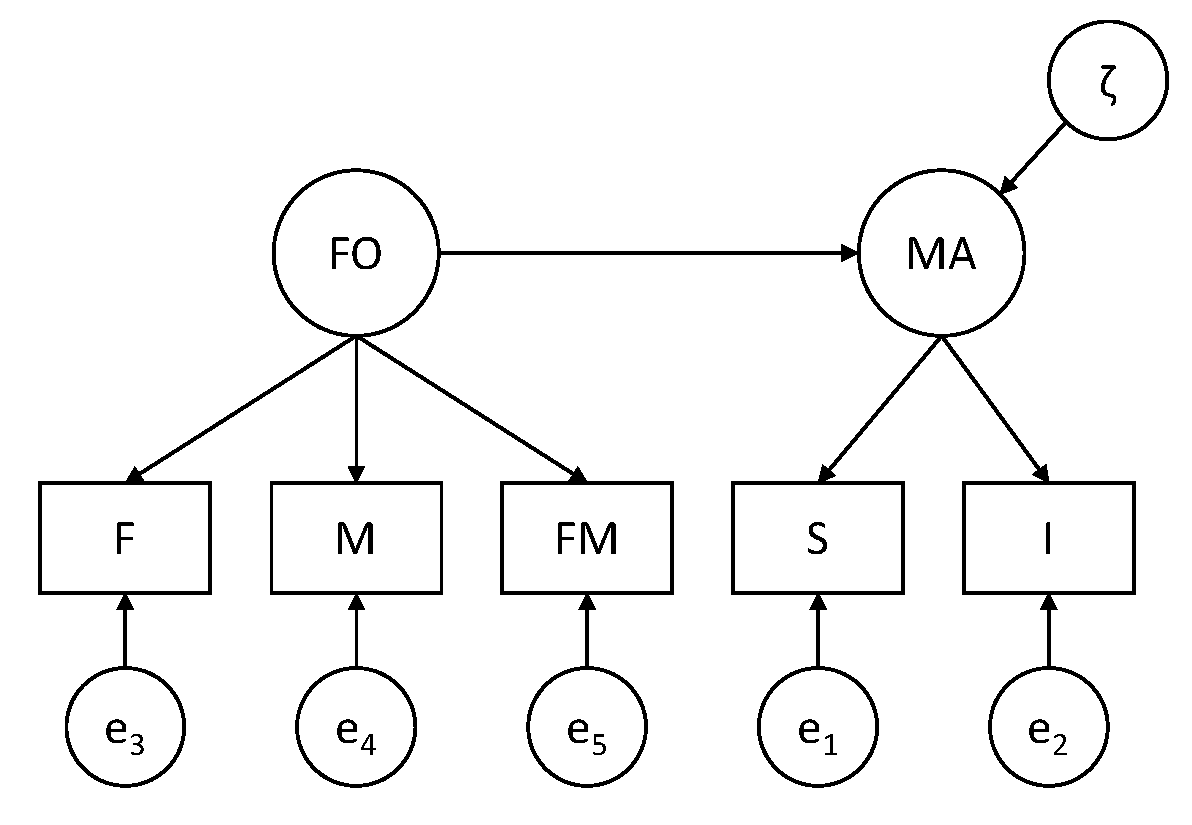
The idea is that the first two variables measure Marital Adjustment (MA) and the latter three variables measure the quality of relationships in the Family of Origin (FO). Furthermore, it is assumed that FO is a predictor of MA.
Question 1
Draw the path diagram for this structural equation model.
Measurement part of the model: S and I are indicators of MA; F, M, and FM are indicators of FO. Structural part of the model: MA is regressed on FO.
Before doing the actual model that includes the structural relation between the latent variables, we start with only the measurement model; this means that we specify a two-factor model in which the latent variables are allowed to covary (i.e., a two-headed arrow between MA and FO). We use this model to investigate whether strong factorial invariance holds by testing whether the assumptions of this model hold.
Question 2
The data for this exercise are included in the file named Family.dat; note it only contains the summary statistics, that is, it contains the means, standard deviations, and correlation matrices for each group (men first, then women), that were printed in the original paper. Have a look at these.
You can open the data either in Mplus, or with a program like notepad. This is what you see:
161.779 138.382 86.229 86.392 85.046
32.936 22.749 13.390 13.679 14.382
1
.740 1
.265 .422 1
.305 .401 .791 1
.315 .351 .662 .587 1
155.547 137.971 82.764 85.494 81.003
31.168 20.094 11.229 11.743 13.220
1
.658 1
.288 .398 1
.171 .295 .480 1
.264 .305 .554 .422 1
Question 3
Typically when you have data, you will have the raw data. In that case you will have the observed variables and a grouping variable in one file. See example 5.14 in the Mplus Users Guide for how to specify the DATA and VARIABLE commands in that case.
Here we only have the summary data. To specify the DATA and VARIABLE commands in this case, use:
DATA:   NGROUPS ARE 2;
        TYPE IS MEANS STD CORR;
        FILE IS Family.dat;
        NOBSERVATIONS ARE 103 103;

VARIABLE:   NAMES ARE S I F M FM;
We will begin with using the automatic option in Mplus that allows us to run all three models that are needed to investigate measurement invariance. This can be done by adding:
ANALYSIS: MODEL = CONFIGURAL METRIC SCALAR;where CONFIGURAL is the model without any constraints across the groups; METRIC is the model we refer to as weak factorial invariance, that is, equal factor loadings across groups; and SCALAR is what we refer to as strong factorial invariance, that is, equal factor loadings and intercepts across groups, and freely estimated latent means in group 2 (and subsequent groups, if there are any).
Use the code above, and add:
TITLEcommandMODELcommand, in which you just specify the general factor model (so no need to specify separate models for separate groups!)OUTPUTcommand
Run the model and check the output. Describe what you see.
In the top menu in Mplus you can change the format of the output file by going to Mplus and choosing HTML output, and then run the model. This will result in output with links that makes it easier to navigate through it. At the beginning of the output, you get to see:
OUTPUT SECTIONS

Input Instructions
Input Warnings And Errors
Summary Of Analysis
Sample Statistics
Model Fit Information
- For The Configural Model
- For The Metric Model
- For The Scalar Model
Model Results
- For The Configural Model
- For The Metric Model
- For The Scalar Model
Technical 1 Output
- For The Configural Model
- For The Metric Model
- For The Scalar Model
Technical 9 Output
Hence, we see that for each of the three models we get information about model fit, we get the parameter estimates, and the additional output (here, we asked for TECH1). We also get TECH9 which contains the warnings for the three models.
While this automatic option is of course very convenient in practice, we will now focus in this exercise on how to specify and run these three models ourselves. The point of this is that we see how we can overrule defaults in Mplus, and we consider the models one by one (and check the TECH1 output), and consider alternative ways of scaling these models.
Step 1: Configural invariance
Question 4
If we specify the model for configural invariance:
- how many sample statistics are there?
- how many free parameters are there?
- how many df are there?
Sample statistics. We have 5 observed variables in each group. Hence, we have 5*6/2 = 15 unique elements in the covariance matrix S for each group, plus 5 observed means, so 20 sample statistics per group. That makes 40 sample statistics in total.
Free parameter. In each group we estimate:
- 3 factor loadings (there are 5 factor loadings, but 2 are used for scaling)
- 2 factor variances
- 1 factor covariance
- 5 residual variances
- 5 intercepts
That makes 16 parameters per group; hence, 32 free parameters in total.
Degrees of freedom. The degrees of freedom are therefore: \(df = 40 - 32 = 8\).
Question 5
Specify the two-factor model for configural invariance.
MODEL:      MA BY S I;
            FO BY F M FM;

MODEL g2:   MA BY S@1 I;
            FO BY F@1 M FM;
            [S I F M FM];
            [MA@0 FO@0];
where the first MODEL: command is the general model specification, and the second part MODEL g2; is overruling the multiple group factor analysis defaults through:
- freeing the factor loadings (so they are not identical to the factor loadings in g1), and using
@1to ensure the factors are scaled - freeing the intercepts in the second group (so they are not identical to the intercepts in g1)
- fixing the latent means to zero (to ensure identification)
Alternatively, one could also say:
MODEL:      MA BY S I;
            FO BY F M FM;

MODEL g2:   MA BY I;
            FO BY M FM;
            [S I F M FM];
            [MA@0 FO@0];
Here, we are doing the same thing, but not overruling the default for the factor loadings of the first indicator of each latent variable (hence the initial scaling remains in tact).
In addition to this MODEL command, we specify the OUTPUT command as:
OUTPUT: TECH1 MOD(4);Question 6
Run this model, and check whether the TECH1 output matches your answer under Question 4 regarding where the free parameters are. Also check the warning(s); is there a reason for concern?
We get this warning:
THE MODEL ESTIMATION TERMINATED NORMALLY

WARNING:  THE RESIDUAL COVARIANCE MATRIX (THETA) IN GROUP G1 IS NOT
POSITIVE DEFINITE.  THIS COULD INDICATE A NEGATIVE VARIANCE/RESIDUAL
VARIANCE FOR AN OBSERVED VARIABLE, A CORRELATION GREATER OR EQUAL TO ONE
BETWEEN TWO OBSERVED VARIABLES, OR A LINEAR DEPENDENCY AMONG MORE THAN TWO
OBSERVED VARIABLES.  CHECK THE RESULTS SECTION FOR MORE INFORMATION.
PROBLEM INVOLVING VARIABLE I.
This implies that the residual covariance matrix contains a combination of numbers (i.e., parameter estimates) that are not possible in a covariance matrix. We can start with checking the relevant parameter estimates in the first group:
Residual Variances
  S                528.470    130.512      4.049      0.000
  I                -39.883    109.198     -0.365      0.715
  F                 21.613     10.983      1.968      0.049
  M                 53.509     11.710      4.570      0.000
  FM               103.074     16.168      6.375      0.000
It shows that the residual variance for the indicator I (intimacy) is negative; this is not possible (as variances are by definition zero or larger). This is referred to as a Heywood case, and is typically interpreted as meaning that the model is too complicated for the data (for instance because the model is really wrong, or because the sample size is too small). I is an indicator of MA, which only has one other indicator (i.e., S); this is often a difficult situation in terms of estimation.
One action we could take is setting this residual variance to zero (note the parameter is not significantly different from zero). That would mean this variable is a perfect indicator of the latent variable MA, as there would be no measurement error at all; this would in turn mean we only need this indicator, and there is no need for the second indicator to measure the latent variable.
But for now, we will just leave the variable in, and consider the model fit before moving on to testing weak factorial invariance.
Question 7
For now, we ignore this warning. What is the model fit?
Chi-Square Test of Model Fit

          Value                              6.025
          Degrees of Freedom                     8
          P-Value                           0.6444
The chi-square test indicates the model fits well (note btw that the degrees of freedom are indeed 8). We see this chi-square is simply the sum of the chi-squares that are obtained for each group, as presented in the output:
Chi-Square Contribution From Each Group

          G1                                 4.688
          G2                                 1.337
The other fit measures also indicate the model fits very well:
RMSEA (Root Mean Square Error Of Approximation)

          Estimate                           0.000
          90 Percent C.I.                    0.000  0.095
          Probability RMSEA <= .05           0.786

CFI/TLI

          CFI                                1.000
          TLI                                1.000

SRMR (Standardized Root Mean Square Residual)

          Value                              0.019
Step 2: Weak factorial invariance
Question 8
Next, specify the model for weak factorial invariance. How many df would this model have? Run this model and report on the model fit.
In the model for weak factorial invariance, we set the factor loadings invariant across groups, while not constraining the mean structure. In practice, this implies we no longer have to overrule the defaults for the factor loadings, but we still need to overrule the defaults for the intercepts and latent means. Hence, the model specification becomes:
MODEL:      MA BY S I;
            FO BY F M FM;

MODEL g2:   [S I F M FM];
            [MA@0 FO@0];
While in the previous model we were estimating 3 factor loadings in each group (so 6 factor loadings in total), we now estimate 3 factor loadings for both groups. Hence, this model has 3 free parameters less, and thus 3 df more than the model for configural invariance; the df should thus be 8+3=11. This also becomes clear when looking at the TECH1 output of this model (see the numbers that identify the free parameters in the matrix LAMBDA).
We see this in the chi-square test:
Chi-Square Test of Model Fit

          Value                              8.735
          Degrees of Freedom                    11
          P-Value                           0.6463
We see indeed the number of df is 11.
Question 9
Do a chi-square difference test to determine whether the assumption of weak factorial invariance (i.e., equal factor loadings across groups) holds.
\(\Delta \chi^2 = 8.735 - 6.025 = 2.710\)
\(\Delta df = 11 - 8 = 3\)
Hence, the chi-square difference is 2.710 with df=3. The p-value for this is 0.4385 (for an online chi-square calculator, see for instance: https://www.fourmilab.ch/rpkp/experiments/analysis/chiCalc.html).
This means that our H0 (i.e., weak factorial invariance) is not rejected. Put differently, the constraints for weak factorial invariance can be imposed.
Step 3: Strong factorial invariance
Question 10
Next, specify the model for strong factorial invariance. Again, indicate how many df this model will have, run the model, and report on the model fit.
Strong factorial invariance is the default multiple group factor model that Mplus runs. Hence, it does not require us to overrule any of its defaults. Compared to the previous model, this means that it will constrain all five intercepts to be identical across the two groups, but at the same time, it will freely estimate the two latent means in the second group. Hence, the difference in df is 5-2=3; the new model with have 3 df more than the one we had before.
The MODEL command for this model is very simple; we only need:
MODEL:      MA BY S I;
            FO BY F M FM;
The chi-square of this model is:
Chi-Square Test of Model Fit

        Value                             15.647
        Degrees of Freedom                    14
        P-Value                           0.3354
We see that indeed the df are 3 more than before (\(11 + 3 = 14\)).
Question 11
Do a chi-square difference test to determine whether the assumption of strong factorial invariance (i.e., equal intercepts; only latent mean differences) holds.
We compare the current model fit to that of the previous model (i.e., the one for weak factorial invariance), to determine whether the additional constraints are tenable.
Hence we have:
\(\Delta \chi^2 = 15.647 - 8.735 = 6.912\)
\(\Delta df = 14 - 11 = 3\)
A chi-square difference test of 6.912 with 3 df has a p-value of 0.0748. Hence, again, the H0 is not rejected, which now means we can assume that strong factorial invariance holds.
Question 12
Check the TECH1 output for the latter model. How do you see the constraints that were imposed?
You can see the intercepts and factor loadings are constrained across the two groups, because the same numbers are used to show which ones are estimated freely:
         NU
            S             I             F             M             FM
           ________      ________      ________      ________      ________
                1             2             3             4             5


         LAMBDA
           MA            FO
            ________      ________
 S                  0             0
 I                  6             0
 F                  0             0
 M                  0             7
 FM                 0             8
Alternative way of scaling
Above, we have used the usual way of scaling:
- first factor loading of each latent variable fixed to 1 (in each group)
- all latent means fixed to 0 (in each group), combined with estimating the intercepts for the observed variables freely (in each group)
In this case, the step from configural to weak factorial invariance now consists of only adding more constraints, which makes it easy to see these two models are nested (i.e., the model for weak factorial invariance is nested under the model for configural invariance).
However, it is less obvious that the model for strong factorial invariance is nested under the model for weak factorial invariance, because it includes constraining parameters (i.e., the intercepts have to be equal across groups), but also requires freeing parameters (i.e., the latent means in the second group are freed).
To ensure that these models are nested, we use an alternative way of specifying these models, based on a different way of scaling. The key issue here is that these alternative model specification are simply reparameterizations of the the same models; they are equivalent models, as we can see because they lead to the exact same model fit.
Question 13
Instead of scaling with the latent means fixed to zero and the intercepts all estimated freely, scale the latent variable in the model for configural invariance through setting the intercept for the first indicator to zero, while allowing the latent mean to be estimated freely. Compare the model fit to the one obtained above for the configural invariance model.
The MODEL command can be specified as:
MODEL:        MA BY S I;
              FO BY F M FM;

MODEL g1:     [S@0 F@0];
              [MA FO];

MODEL g2:     MA BY S@1 I;
              FO BY F@1 M FM;
              [S@0 I F@0 M FM];
When running the model like this, it does not converge within the default number of iterations. We get this message:
NO CONVERGENCE. NUMBER OF ITERATIONS EXCEEDED.and there is no model fit, standard errors, or p-values. This can mean the model is too complicated. It can also mean you need to specify (better) starting values. As a first step, we can just increase the number of iterations, by adding:
ANALYSIS: ITERATIONS ARE 20000;In this case, this solves it, that is, the model now converges. When considering the model fit, we see it is exactly the same as that of the model discussed in Question 7.
Chi-Square Test of Model Fit

          Value                              6.025
          Degrees of Freedom                     8
          P-Value                           0.6444
Because the chi-square is exactly the same (and the df), this implies these models are statistically equivalent; they are identical, just parameterized differently. You cannot distinguish between them on statistical grounds.
Hence, this shows that this alternative way of scaling the latent variables gives a model that is equivalent.
Question 14
Next, use this alternative way of scaling and specify the model for weak factorial invariance.
The MODEL command can be specified as:
MODEL:        MA BY S I;
              FO BY F M FM;

MODEL g1:     [S@0 F@0];
              [MA FO];

MODEL g2:     [S@0 I F@0 M FM];
That is, we no longer overrule the defaults for the factor loadings. Note that for this model to converge, we do not need to increase the number of iterations.
When considering the model fit, we see it is exactly the same as that of the model discussed in Question 8:
Chi-Square Test of Model Fit

          Value                              8.735
          Degrees of Freedom                    11
          P-Value                           0.6463
This means that the current model is statistically equivalent to the model we had before to impose weak factorial invariance.
Question 15
And now, the Moment Suprême: We will specify the model for strong factorial invariance using this alternative way of scaling. The key issue to notice here is that in going from weak factorial invariance to strong factorial invariance, we will now only add constraints, which makes it very clear that the latter model must be nested under the former.
Remember that before, we were adding constraints (i.e., fixing the intercepts to be identical across the groups), but also were freeing parameters (i.e., allowing the latent means in the second group to be estimated freely); this makes it difficult to see that the model for strong factorial invariance is nested under that of weak factorial invariance.
But with this alternative way of scaling, which leads to statistically equivalant models (i.e., models with the exact fit, and which are thus indistinguishable), we now only add constraints on parameters when going from weak to strong factorial invariance, such that it is very obvious that (and how) they are nested.
Specify the model for strong factorial invariance using this alternative way of scaling.
The MODEL command can be specified as:
MODEL:        MA BY S I;
              FO BY F M FM;

MODEL g1:     [S@0 F@0];
              [MA FO];

MODEL g2:     [S@0 F@0];
This model leads to the exactly same model fit as that of the model discussed in Question 10:
Chi-Square Test of Model Fit

          Value                             15.647
          Degrees of Freedom                    14
          P-Value                           0.3354
This means that the current model is statistically equivalent to the model we had before to impose strong factorial invariance. This also means that we can now be certain that the model for strong factorial invariance is nested under the model for weak factorial invariance; this means we can do a chi-square difference test to compare them (as we already did above).
Question 16
While this alternative way of specifying the series of models is useful to seeing their nestedness, the first way of specifying the models also has advantages. One of these advantages is that it requires fewer defaults to be overruled. But more importantly, it allows us to easily determine in the strong factorial invariance model whether there are latent mean differences between the groups. Report and interpret these.
In the first approach, the model for strong factorial invariance is based on constraining the factor loadings and intercepts across the groups, and freeing the latent means in the second group, while the means in the first group are fixed to zero.
That is, for G1 we get:
Means
    MA                 0.000      0.000    999.000    999.000
    FO                 0.000      0.000    999.000    999.000
and for G2 we get:
Means
    MA                -0.415      3.118     -0.133      0.894
    FO                -3.140      1.655     -1.898      0.058
This implies that the significance test of the latter can be used to determine whether there are latent mean differences between the second and the first group. Here we get a p-value of 0.894 for MA, and a p-value of 0.058 for FO; hence for both we do not find evidence that they differ from zero, which means that for both we do not find evidence that the two groups differ.
Full model
As both the test for weak and for strong factorial invariance were non-significant, we can conclude that strong factorial invariance holds. This means we can compare individuals from these groups, and we can compare the means of these groups. It also means that the constructs “Marital Adjustment” and “Family of Origin” are measured in the same way in these two groups, and that we can specify a structural model for these latent variables in the two groups to investigate how they are related.
Question 17
Specify the model as initially intended, with FO as a predictor of MA at the latent level, while assuming strong factorial invariance.
The model is now specified as:
MODEL:      MA BY S I;
            FO BY F M FM;
            MA ON FO;
Question 18
Run this model, and compare the model fit to that of the model for strong factorial invariance that we had before. What do you conclude?
These models have the exact same model fit (same chi-square and df). This means these models are statistically equivalent. Hence, it does not matter whether you estimate the covariance between the two latent variables, or a regression coefficient.
Question 19
When comparing the TECH1 output of these two models, what difference do you spot?
In the two-factor model we have for G1:
          BETA
              MA            FO
              ________      ________
 MA                 0             0
 FO                 0             0


           PSI
              MA            FO
              ________      ________
 MA                14
 FO                15            16
that is, no structural parameters, and a covariance is Psi; in contrast in the regression model we have for G1:
               BETA
                  MA            FO
                  ________      ________
     MA                 0            14
     FO                 0             0


               PSI
                  MA            FO
                  ________      ________
     MA                15
     FO                 0            16
showing there is a structural parameter in Beta (going to MA, coming from FO), and there is no covariance estimated in Psi. The same is true for G2.
Question 20
As a final step, we want to investigate whether the regression coefficient is different in the two groups or not. How can you investigate this?
In the model above, the regression parameter was not constrained across the groups. We can now specify a model in which we constrain the parameter to be invariant across the two groups; that model will be nested under the previous model, and we can thus do a chi-square difference test to see whether the constraint holds.
To constrain the parameter across the groups, we only have to give it a label (i.e., a name). Here we will give it the label c (you could als give it a longer name, such as coeff). The model is now specified as:
        MODEL:      MA BY S I;
                    FO BY F M FM;
                    MA ON FO (c);
To see that this leads to having the same regression coefficient in both groups, we can check the TECH1 output. For G1 we have (only showing part of it):
           ALPHA
              MA            FO
              ________      ________
                    0             0


           BETA
               MA            FO
              ________      ________
 MA                 0            14
 FO                 0             0


          PSI
             MA            FO
              ________      ________
 MA                15
 FO                 0            16
and for G2:
         ALPHA
             MA            FO
             ________      ________
                  22            23


          BETA
              MA            FO
              ________      ________
 MA                 0            14
 FO                 0             0


           PSI
              MA            FO
              ________      ________
 MA                24
 FO                 0            25
It shows that the structural parameter in both cases is the same parameter (number 14).
The model fit is:
Chi-Square Test of Model Fit

          Value                             16.315
          Degrees of Freedom                    15
          P-Value                           0.3614
showing it has 1 df more than the model we had before (because we estimate 1 parameter less). Doing a chi-square difference test we get:
\(\Delta \chi^2 = 16.315 - 15.647 = 0.688\) with \(df-1\), which gives a p-value of 0.4137, which means the test is not significant. Hence, H0 does not have to be rejected, and we can therefore assume that the regression coefficient is identical across the two groups.
Conclusion
To summarize what we did in this exercise:
- we were interested in investigating a full SEM model (with both a measurement model and a structural model), in two groups
- before we could investigate the structural part of the model (i.e., the latent regression), we had to determine whether there was measurement invariance across the groups
- to this end we ran a series of three models: configural invariance, weak factorial invariance and strong factorial invariance; these models are increasingly more restrictive, and we compared each subsequent model with the preceding one (using a chi-square different test) to see whether the additional constraints were tenable
- since neither of the two chi-square difference test reached significance, we can conclude that strong factorial invariance holds; this means we are measuring the same constructs in both groups, and we can compare their latent means
- we also considered an alternative way to scale the models (based on setting one of the intercepts per factor to zero, rather than the latent means), which more clearly shows that the model for strong factorial invariance is a special case of the model for weak factorial invariance
- the first way of scaling has the advantage that we can immediately see whether the means of the two groups on the latent variables differ or not; here we found no significant difference
- since the latent variables are measured in the same way in both groups, we continue with our actual research question, which concerns the latent regression model; regressing the latent variables on each other resulted in a model that is equivalent to the model for strong factorial invariance
- subsequently, we constrained the regression coefficient across the two groups to see whether the effect of family of origin (FO) has the same effect on marital adjustment (MA) in the two groups; again, by doing a chi-square difference test we could determine whether or not this constraint was tenable; since the test was not significant, we may assume that the two regression slopes are the same across the groups
- note that in the end, we still have the same warning as for the first model about a Heywood case (negative variance) in the first group; we should present such results in a paper; we could constrain this variance to zero (and we could do the same thing in the other group, because it is not significantly different from zero there either), which would make this indicator and the latent variable it measures identical; put differently, this implies that we can measure marital adjustment with this one variable, and we do not need the other one for it
Path analysis
In this exercise, we consider a path model in which observed variables are regressed on each other. The data come from the paper Hale et al. (2005). We collected the means, standard deviations, and correlation matrix from that paper for the group of older boys (n=275) in the file BoysDep.dat. We have the following four variables (in this order):
- perceived parental rejection (PPR)
- adolescent depression (AD)
- adolescent aggression (AA)
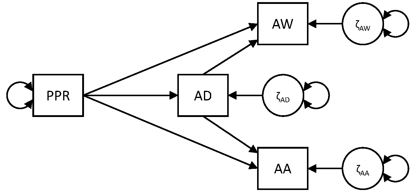
- adolescent withdrawal (AW)
The model that the researchers proposed, is presented below: Their question is whether perceived parental rejection (meaning the adolescent feels rejected by the parents), leads adolescents to feel sad (as operationalized with adolescent withdrawal), or mad (as operationalized with adolescent aggression), and to what extent these effects are mediated through adolescent depression.
Question 1
Determine: a) how many sample statistics there are; b) how many free parameters there are: and c) how many degrees of freedom this model has.
There are four observed variables, so \(\frac{4 \times 5}{2} = 10\) unique elements in the covariance matrix S, and 4 observed means; that makes 14 sample statistics in total.
The number of free parameters in this model are: 1 variance of the exogenous variable (PPR), 3 residual variance of the endogenous variables (AD, AA and AW), 5 structural parameters (i.e., regression coefficients), 1 mean for the exogenous variable (PPR), and 3 intercepts for the endogenous variables (AD, AA, and AW). That makes 13 free parameters in total.
The number of degrees of freedom should therefor equal \(14 - 13 = 1\).
Question 2
To specify the above model, make use of this code for the DATA command:
DATA:       TYPE IS MEANS STDEVIATIONS CORRELATION;
            FILE = BoysDep.dat;
            NOBSERVATIONS = 275;
Note that when we have summary data, we have to tell Mplus how many observations there are, because it is not possible to know this in any other way.
Also, make use of this code for the MODEL command:
MODEL:      AD ON PPR;
            AA ON AD PPR;
            AW ON AD PPR;
Finish the code and run the model. Consider the model fit results: Do they make sense to you?
Below are the two most notable parts of the model fit output.
MODEL FIT INFORMATION

Number of Free Parameters                       12

...

Chi-Square Test of Model Fit

          Value                              0.000
          Degrees of Freedom                     0
          P-Value                           0.0000
It indicates that there are 12, rather than 13, free parameters, and that there are 0, rather than 1, degree of freedom. At first sight, this makes no sense: 12+0=12, but this should equal the number of sample statistics, which we determined is 14.
Question 3
There are actually two things going on at once here. Check the TECH1 output to see whether you can figure out what the two issues are.
Considering the first three matrices in TECH1:
TECHNICAL 1 OUTPUT

     PARAMETER SPECIFICATION

           NU
              AD            AA            AW            PPR
              ________      ________      ________      ________
                  0             0             0             0

           LAMBDA
              AD            AA            AW            PPR
              ________      ________      ________      ________
 AD                 0             0             0             0
 AA                 0             0             0             0
 AW                 0             0             0             0
 PPR                0             0             0             0


           THETA
              AD            AA            AW            PPR
              ________      ________      ________      ________
 AD                 0
 AA                 0             0
 AW                 0             0             0
 PPR                0             0             0             0
These three matrices are associated with the measurement equation and contain no free parameters for a path model.
Consider the second set of three model matrices:
           ALPHA
              AD            AA            AW            PPR
              ________      ________      ________      ________
                  1             2             3             0


           BETA
              AD            AA            AW            PPR
              ________      ________      ________      ________
 AD                 0             0             0             4
 AA                 5             0             0             6
 AW                 7             0             0             8
 PPR                0             0             0             0


           PSI
              AD            AA            AW            PPR
              ________      ________      ________      ________
 AD                 9
 AA                 0            10
 AW                 0            11            12
 PPR                0             0             0             0
Here we see where the free parameters are (adding up to 12, which was the number indicated in the Mplus output). There are three things to notice here:
- the order of the variables has been changed by Mplus, and the exogenous variable PPR is placed at the end in these matrices; this may be somewhat inconvenient when looking at these matrices, but is not a problem
- the mean and the variance for this exogenous variable are not counted as free parameters; this is because they are exactly the same as the observed mean and variance, which in turn are not counted as sample statistics (hence, the free parameters + df add up to 12 rather than 14); while this does not affect model fit here, we can decide to overrule this, asking for the means and/or variance of PPR, which changes its status to endogenous
- there is a covariance between the residuals of AW and AA (the off-diagonal element, parameter 11 in the Psi matrix); apparently, this is a default that Mplus imposes for path models, that the variables at the end (i.e., the endogenous variables that are only dependent variables, and do not predict anything themselves) have correlated residuals; if we don’t want that, we have to actively set this covariance to zero
Regarding the latter point, we may also look at the parameter estimate for this covariance:
         AW       WITH
            AA                 1.173      1.358      0.864      0.388
This covariance is not significantly different from zero; hence, we can decide that it can be omitted from the model (which is the same as fixing it to zero).
Question 4
Specify a model that overrules the defaults we ran into in the previous question. Discuss the model fit. Check the TECH1 output and notice the differences with what you saw before.
We use the following MODEL command:
MODEL:      AD ON PPR;
            AA ON AD PPR;
            AW ON AD PPR;
            AA WITH AW@0;
            PPR;
The fit information we get with this code is:
MODEL FIT INFORMATION

Number of Free Parameters                       13

  ...

Chi-Square Test of Model Fit

          Value                              0.750
          Degrees of Freedom                     1
          P-Value                           0.3865
So now we see there are 13 free parameters in this model and there is 1 df; this is what we determined in the beginning (and \(13 + 1 = 14\), so it nicely adds up to the total number of sample statistics that we counted to begin with).
When checking the TECH1 output, what we notice is:
- the free parameters are counting up to 13
- the mean and variance of the exogenous variable PPR are now both counted as free parameters
- the covariance between the residuals of AA and AW is no longer estimated (not a free parameter)
Question 5
We are actually interested not so much in overall model fit here (the model has only 1 df, so it is very unlikely that will not fit well), but rather in its parameter estimates, and even more so, in the mediated and direct effects.
To get information about the indirect (i.e., mediated) effects, we have to add these lines to the code:
        MODEL INDIRECT:
                    AA IND PPR;
                    AW IND PPR;
Run the model with this code added, and report on the indirect effects.
Note that the model itself has not changed (you can also tell by the fact that the model fit and parameter estimates are the same as before); we just have additional output.
The nonstandardized additional output starts with:
TOTAL, TOTAL INDIRECT, SPECIFIC INDIRECT, AND DIRECT EFFECTS

                                                    Two-Tailed
                    Estimate       S.E.  Est./S.E.    P-Value

Effects from PPR to AA

  Total                0.538      0.247      2.174      0.030
  Total indirect       0.221      0.085      2.608      0.009

  Specific indirect 1
    AA
    AD
    PPR                0.221      0.085      2.608      0.009

  Direct
    AA
    PPR                0.317      0.240      1.320      0.187
It reports all there is to know about the effect of PPR on AA:
- the direct effect is not significant (\(p = .187\))
- the indirect effect through AD is significant and positive (\(p = .009\)), meaning that higher perceived parental rejection leads to higher aggression
- the total indirect effect is the same, as there is only one indirect effect (there can be multiple indirect through different series of mediators in more complicated models)
- the total effect is the total indirect effect (i.e., all indirect effects) plus the direct effect
Because the direct effect is not significant, we could decide to take this out of the model (which is the same as setting it to zero).
For the second outcome variable we get:
Effects from PPR to AW

  Total                0.035      0.070      0.498      0.619
  Total indirect       0.042      0.019      2.249      0.025

  Specific indirect 1
    AW
    AD
    PPR                0.042      0.019      2.249      0.025

  Direct
    AW
    PPR               -0.007      0.070     -0.103      0.918
Pretty much the same picture: The direct effect is non-significant and could thus be fixed to zero. The indirect effect is significantly different from zero, and positive, meaning more perceived parental rejection is followed by more adolescent withdrawal.
We can also look at the standardized effects, but let’s first fix the non-significant direct effects to zero.
Question 6
Fix the non-significant direct effects to zero, and run the model again. Consider the standardized indirect effects in this model: What can you conclude with regard to the researchers’ question: Does perceived rejection make adolescents sad or mad?
The standardized indirect effect of PPR on AA is:
          Specific indirect 1
            AA
            AD
            PPR                0.056      0.021      2.680      0.007
The standardized indirect effect of PPR on AW is:
          Specific indirect 1
            AW
            AD
            PPR                0.036      0.016      2.281      0.023
We see the effect of PPR on AA (aggression) is larger than that on AW (withdrawal). Hence, we could say that perceived parental rejection makes adolescents more mad than sad, although it also makes them sad. Note however that these effects are both quite small.
Question 7
Consider the parameter estimates from the non-standardized solution and write down the regression equations for the three dependent variables in the model; fill in the actual parameter estimates for the intercepts and slopes (i.e., regression coefficients).
For adolescent depression we have:
\[AD_i = 22.096 + 0.609*PPR_i + \zeta_{ADi}\]
For adolescent aggression we have:
\[AA_i = 16.739 + 0.379*AD_i + \zeta_{AAi}\] \[ = 16.739 + 0.379*(22.096 + 0.609*PPR_i + \zeta_{ADi})+ \zeta_{AAi}\]
For adolescent withdrawal we have:
\[AW_i = 6.842 + 0.0.069*AD_i + \zeta_{AWi}\] \[= 6.842 + 0.069*(22.096 + 0.609*PPR_i + \zeta_{ADi})+ \zeta_{AWi}\]
Conclusion
When doing a path analysis with only observed variables, there are several defaults that are operating. It can be helpful to check the TECH1 output to see what and where they are (rather than trying to memorize all of them).
Some aspects regarding observed exogenous variables to keep in mind:
- observed exogenous variables are observed variables that do not have any one-headed arrows pointing towards them; this means that they are not predicted by anything
- Mplus treats such variables differently than other variables; specifically: a) their observed variances, covariances and means are not counted as sample statistics; and b) their estimated variances, covariances and means are not counted as free parameters; note these two cancel each other out (in terms of sample statistics - free parameters = degrees of freedom)
- When there are no missing data, the observed means, variances and covariances for observed exogenous variables are identical to their estimated means, variances and covariances
- When there are missing data, Mplus will use case-wise deletion for cases that have missings on the observed exogenous variables; this may be undesirable, and can be avoided by changing the status of these variables in Mplus to endogenous by asking for their means and/or variances (then Mplus will keep all cases and use ML to deal with the missing observations)
- Another scenario in which we need to be concerned about observed exogenous variables being treated differently, is when we want to compare such a model to a model in which one or more of these variables are not exogenous; the AIC and BIC of these two models will not be comparable; you can tell by looking at the loglikelihood value for H1 (i.e., for the saturated model), just above the
Information Criteriain the output; if these are not the same, the AIC and BIC are not comparable!
Some issues regarding additional defaults to keep in mind:
- In a path model with observed variables only, you have exogenous variables and endogenous variables; the latter can be further distinguished into mediators (i.e., they are dependent variables, but also predictors of other variables), and outcome variables (i.e., they have only arrows pointing towards them, not out of them)
- The exogenous variables in such models are by default allowed to covary (i.e., there is a two-headed arrow between them); typically, that is fine as we do not have a specific theory about how the predictors are related to each other; however, if you do not want them to be correlated, you can set their covariance to zero with the
WITHstatement (note this will also change their status from exogenous to endogenous) - The residuals of mediators in such models are uncorrelated, unless you specify they should covary (using the
WITHstatement) - The residuals of outcome variables in such models are by default allowed to be correlated (or: to covary); in terms of a path diagram this implies Mplus automatically adds a two-headed arrow between these residuals
- You can use the
TECH1output to trace these defaults
Some issues regarding indirect effects to keep in mind:
- In this exercise we let Mplus compute the indirect (i.e., mediated) effects by simply multiplying the parameter estimates; the p-value that is reported for this, is known as the Sobel test; however, it is also known that this test is not correct
- A better approach to determine whether the indirect effect differs from zero or not, is through using bootstrapping and checking the 95% confidence interval for the indirect effect; this can be easily done in Mplus, but requires you to have the raw data (here we only have the summary data, which makes it impossible); in that case you may add to your code:
ANALYSIS:
  BOOTSTRAP = 1000; ! Gives bootstrapped point estimates, standard errors and p-values

OUTPUT:
  CINTERVAL(BOOTSTRAP); ! Gives confidence intervals based on bootstrap (i.e., it can be asymmetric)