Part 1: The quasi-simplex model
Day 4: Cross-lagged relations
In this first part of the computer lab session we will focus on the quasi-simplex model. We are going to study the concept of life satisfaction. The covariance matrix is in the file Coenders.dat and comes from 1724 children and adolescents that participated in the National Survey of Child and Adolescent Well-Being (NSCAW) in Russia. They indicated how satisfied they were with their lives as a whole on a 10-point scale (1 = not at all satisfied, 10 = very satisfied). There were three waves (1993, 1994 and 1995). At the third wave, the question was asked twice (with 40 minutes in between). Hence, in total there are four measurements obtained at three waves. The data and variables commands for these data should read:
DATA:
  TYPE = COVARIANCE;
  FILE = Coenders.dat;
  NOBSERVATIONS = 1724;

VARIABLE:
  NAMES = Y1 Y2 Y3 Y4;
All of the input files for the exercises are provided with the course materials on SURFdrive.
Exercise A
The researchers are interested in fitting a quasi-simplex model to these data, that is, a simplex model at the latent level, thus accounting for measurement error in the observations. This model is graphically represented in the slides. Provide the names of the variances (i.e., indicate in which model matrix, and which position in this matrix they have) in the quasi-simplex graph in the slides. What is the difference between the \(e\)’s and the \(\zeta\)’s?
\(e\)’s are residuals at the measurement level and can be found in the \(\theta\)-matrix. They only influence the observation at a single occasion in time. \(\zeta\)’s are residuals of the simplex process and can be found in the \(\psi\)-matrix. Their effect is carried forward to future observation through the autoregressive relationships. This difference allows Mplus to estimate both types of ``errors’’.
Exercise B
How would you specify the model in Mplus?
See the Mplus input file Exercise B.inp.
Exercise C
Determine the number of degrees of freedom for this model (indicate how you obtained this number). Is it possible to estimate this model?
There are \(\frac{4 \times 5}{2} = 10\) unique elements in \(S\).
Free parameters:
- 4 residual variances at measurement level
- 1 factor variance
- 3 residual factor variances
- 3 regression parameters
- 11 parameters in total.
Therefore, we have \(10 - 11 = -1\) df. It is not possible to estimate this model because we are trying to estimate more parameters than we have information in the data.
Exercise D
To make sure a quasi-simplex model is identified, often the variances of the measurement errors are constrained to be equal over time. How can you do this in Mplus? How many df does this model have?
See the Mplus input file Exercise E.inp for how to constrain the measurement error variances over time. With constrained measurement error variances, we estimate 3 parameters less. So, we estimate \(11 - 3 = 8\) and therefore have \(10 - 8 = 2\) df.
Exercise E
Run the model and report on the model fit.
We find the below fit indices:
- \(\chi^{2}\) = 13.29 with df = 2, \(p = .0013\),
- RMSEA = .057,
- CFI = .994, and
- TLI = .981.
Except for \(\chi^{2}\) test of model fit, the model seems to fit the data well. Note, however, that the sample size is very large and therefore the \(\chi^{2}\) is likely to be significant, even for minor problems with model fit.
Exercise F
The quasi-simplex model you just ran, led to the following warning:
WARNING: THE LATENT VARIABLE COVARIANCE MATRIX (PSI) IS NOT POSITIVE DEFINITE.
THIS COULD INDICATE A NEGATIVE VARIANCE/RESIDUAL VARIANCE FOR A LATENT VARIABLE,
A CORRELATION GREATER OR EQUAL TO ONE BETWEEN TWO LATENT VARIABLES, OR A LINEAR
DEPENDENCY AMONG MORE THAN TWO LATENT VARIABLES. CHECK THE TECH4 OUTPUT FOR MORE
INFORMATION. PROBLEM INVOLVING VARIABLE ETA4.
What is the problem?
In your output, look at the reported (estimated) residual variances. We find that the residual variance of ETA4 is estimated to be negative. This is a Heywood case and it is causing the warning to appear. Note however, that it is significant, so ``just” fixing it to 0 as a solution is probably not warranted here.
Exercise G
As indicated in the description of the data, the third and fourth measurement were obtained at the same measurement wave (with only 40 minutes in between). Hence, the researchers proposed the following model instead of the regular quasi-simplex model. Explain why this model makes more sense for these data than the regular quasi-simplex model. Tip: check the description of the study at the beginning of this exercise.
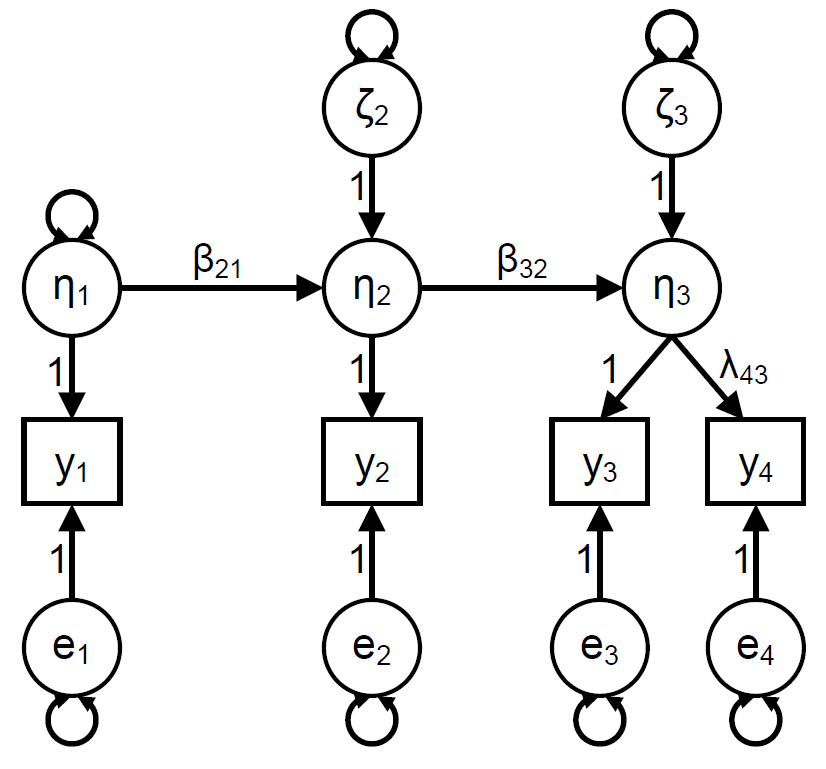
At each occasion there is a latent variable which represents Life Satisfaction. At the first two occasions there was only a single indicator of this latent variable, but at the third occasion there were two indicators.
Exercise H
How many df does this model have? Note that we keep the constraint on the variances of the measurement errors.
There are \(\frac{4*5}{2} = 10\) unique elements in S. We freely estimate:
- 1 constrained residual variances at measurement level
- 1 factor variance
- 2 residual factor variances
- 2 regression parameters
- 1 factor loading
- 7 parameters in total.
Therefore, we have \(10 - 7 = 3\) df.
Exercise I
Are these two models nested? If so, how? If not, why not, and how could we compare them?
Yes, they are nested: this model is a special case of the previous model, as it is based on having ETA3 and ETA4 from the previous model now being a single latent variable. That is, we can constrain the residual variance of ETA4 to zero to get the alternative model. This gives us 1 df for the difference.
Exercise J
Specify this model in Mplus and run it. Report on the model fit.
See the Mplus input file Excercise J.inp for the model specification in Mplus. Apart from the \(\chi^{2}\)-test of model fit, the model fits well:
- \(\chi^{2} (3) = 27.37\), with \(p < .001\),
- RMSEA = 0.069,
- CFI = 0.987,
- TLI = 0.973, and
- SRMR = 0.039.
Exercise K
Compare the two models to each other. What can you conclude?
Comparing both models using the \(\Delta \chi^{2}\)-test gives us \(27.37 – 13.29 = 14.0\) with 1 df such that \(p < .001\). This implies that imposing the restriction is not tenable. You can calculate the p-value of the \(\Delta \chi^{2}\) using the pchisq()-function in R (with the lower.tail argument set to FALSE), or an online tool
Comparing the models using information criteria gives us AIC = 29593 and BIC = 29637 for the first model, and AIC = 29605 and BIC = 29643 for the second. In conclusion, all measures indicate the first model is better. However, the current model makes more theoretical sense, and the negative variance estimate in the first model is a problem. For these 2 reasons, we should prefer the current model.
Exercise L
Can you improve the second model in any way? Indicate which parameter you would add to your model, and what this parameter represents in substantive terms.
You can get the modification indices by adding MOD to the OUTPUT command. Here, the suggested BY statements make no sense (later life satisfaction as an indicator of previous life satisfaction). With regards to the ON statement, only the suggested effect of ETA3 ON ETA1 makes sense as we then predict forwards in time. The WITH statement suggests adding a covariance between … (see the next exercise).
Exercise M
Run a model in which you include the Y3 WITH Y4 parameter. Where will this relationship end up in the model? Does it lead to a significant improvement? How would you interpret this additional parameter?
See Exercise M.inp for the Mplus specification of this model. The Y3 WITH Y4 parameter is an additional covariance between the residuals of y3 and y4 (so not between y3 and y4 themselves). If we add this covariance and look at the standardized results, we get a correlation. This correlation actually quite high: \(.522\) (SE = .044), \(p < .001\).
Model fit is quite good (except for the \(\chi^{2}\)-test of model fit):
- \(\chi^{2} (2) = 7.077\), \(p = .0291\),
- RMSEA = 0.038,
- CFI = 0.997,
- TLI = 0.992, and
- SRMR = 0.011.
To compare this model to the previous model, we can do a the \(\Delta \chi^{2}\)-test: \(27.37 – 7.08 = 20.29\), with 1 df such that \(p < .001\), which implies that adding the covariance between the residuals leads to a significant improvement in model fit. This additional parameter implies that y3 and y4 have more in common with each other than what would be expected based on their common dependence on ETA3.