Skip to content

ACCREU damages and adaptation

Back to damage models

During the ACCREU project, new damage estimates were developed for riverine flooding, labour productivity, sea-level rise and mortality. Moreover, adaptation costs and effectiveness were estimated for all sectors (except mortality).

Usage:

params = load_params()
params["model structure"]["damage module"] = "ACCREU"
model = MIMOSA(params)
params = load_params()
params["model structure"]["damage module"] = "ACCREU"
params["economics"]["damages"]["accreu"]["adaptation"] = "sectoral"
model = MIMOSA(params)

By default, only the damages are considered, without adaptation. Adaptation can be enabled with the parameter ACCREU adaptation set to sectoral. If adaptation is enabled, the regional adaptation costs for each sector become additional control variables (either optimised by the solver, or set by the user in simulation mode). The adaptation costs are then used to reduce the damages in sector \(i\) according to the adaptation level:

\[ \text{damages}_{i,t,r} = \text{gross damages}_{i,t,r} \cdot (1 - \text{adapt. level}_{i,t,r}), \]

The adaptation level is calculated as a function of absolute adaptation costs (in currency units) using a negative-exponential saturation (NES) curve:

\[ \text{NES}(\text{adapt. costs}_{i,t,r}; \cdot) = \text{max effectiveness}_{i,r} \cdot \left(1 - e^{-c_{i,r} \cdot \text{adapt. costs}_{i,t,r}}\right) \]
Source code in mimosa/components/damages/accreu/utils.py
def adaptation_effectiveness_fct(adapt_costs, max_effectiveness, cost_param):
    r"""
    The adaptation level is calculated as a function of absolute adaptation costs
    (in currency units) using a negative-exponential saturation (NES) curve:

    $$
    \text{NES}(\text{adapt. costs}_{i,t,r}; \cdot) = \text{max effectiveness}_{i,r} \cdot \left(1 - e^{-c_{i,r} \cdot \text{adapt. costs}_{i,t,r}}\right)
    $$
    """

    return max_effectiveness * (1 - exp(-cost_param * adapt_costs))

Impact sectors

The impacts of riverine flooding are estimated using the GLOFRIS model. The gross damages are fitted with a quadratic function of temperature:

\[ \href{./#var__riverine_damage_costs_gross}{\text{gross damages}_{\text{riverine},t,r}} = (\href{./#param__regional.ACCREU.riverine_noadapt_ead_constant}{a_r} + \href{./#param__regional.ACCREU.riverine_noadapt_ead_linear}{b_r} \cdot \href{./#var__temperature}{T_t} + \href{./#param__regional.ACCREU.riverine_noadapt_ead_quadr}{c_r} \cdot \href{./#var__temperature}{T_t}^2) - (\href{./#param__regional.ACCREU.riverine_noadapt_ead_constant}{a_r} + \href{./#param__regional.ACCREU.riverine_noadapt_ead_linear}{b_r} \cdot \href{./#param__temperature.initial}{T_0} + \href{./#param__regional.ACCREU.riverine_noadapt_ead_quadr}{c_r} \cdot \href{./#param__temperature.initial}{T_0}^2). \]

The adaptation function is fitted with a negative-exponential saturation (NES) curve, like in all three sectors, using regional max. effectiveness and cost coefficient:

\[ \href{./#var__riverine_adaptation_level}{\text{adapt. level}_{\text{riverine},t,r}} = \text{NES}(\href{./#var__riverine_adaptation_costs_abs}{\text{adapt. costs}_{\text{riverine},t,r}}; \href{./#param__regional.ACCREU.riverine_adapt_eff_max_effectiveness}{\text{max eff.}_{\text{riverine},r}}, \href{./#param__regional.ACCREU.riverine_adapt_eff_cost_param}{c_{\text{riverine},r}}) \]

Subsequently, the residual damages are calculated as:

\[ \href{./#var__riverine_damage_costs}{\text{damages}_{\text{riverine},t,r}} = \href{./#var__riverine_damage_costs_gross}{\text{gross damages}_{\text{riverine},t,r}} \cdot (1 - \href{./#var__riverine_adaptation_level}{\text{adapt. level}_{\text{riverine},t,r}}), \]
  • Global damages (without adaptation)


  • Global adaptation costs


Regional damage and adaptation functions
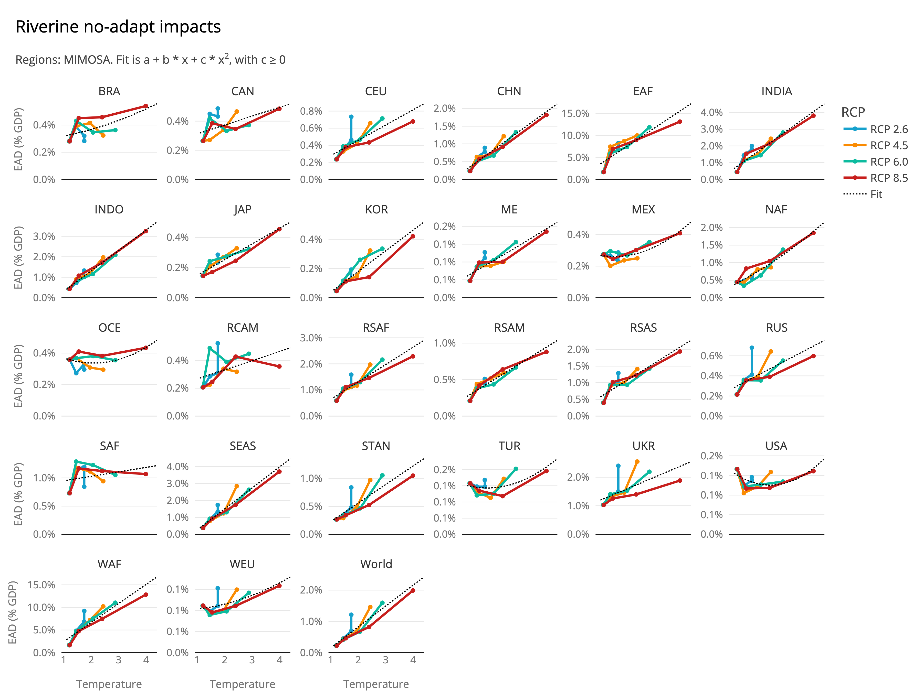
Regional damage costs (without adaptation)

Regional damage costs (without adaptation)

Variables created in this module:
riverine_damage_costs_gross: Gross damages from riverine flooding, without adaptation.
riverine_adaptation_costs_abs: Absolute adaptation costs for riverine flooding, in currency units. Used to calculate the adaptation level.
riverine_adaptation_costs: Adaptation costs for riverine flooding, as a fraction of GDP.
riverine_adaptation_level: Adaptation level for riverine flooding, as a fraction of gross damages. 0 means that no damages are avoided, while 1 means that all damages are avoided.
riverine_damage_costs: Residual damages from riverine flooding, after adaptation. If `noadaptation` is chosen, this variable represents the gross damages.
Source code in mimosa/components/damages/accreu/riverine_flooding.py
def get_constraints(
    m: ConcreteModel, inputs: ModelInputs, adaptation_options: AdaptationOptions
):
    r"""

    The impacts of riverine flooding are estimated using the GLOFRIS model. The gross damages
    are fitted with a quadratic function of temperature:

    :::mimosa.components.damages.accreu.riverine_flooding.gross_dmg_fct_riverine
        options:
            show_source: false

    The adaptation function is fitted with a negative-exponential saturation (NES) curve, like in
    all three sectors, using regional [max. effectiveness](#param__regional.ACCREU.riverine_adapt_eff_max_effectiveness) and [cost coefficient](#param__regional.ACCREU.riverine_adapt_eff_cost_param):

    $$
    \href{./#var__riverine_adaptation_level}{\text{adapt. level}_{\text{riverine},t,r}}
    = \text{NES}(\href{./#var__riverine_adaptation_costs_abs}{\text{adapt. costs}_{\text{riverine},t,r}};
    \href{./#param__regional.ACCREU.riverine_adapt_eff_max_effectiveness}{\text{max eff.}_{\text{riverine},r}},
    \href{./#param__regional.ACCREU.riverine_adapt_eff_cost_param}{c_{\text{riverine},r}})
    $$

    Subsequently, the residual damages are calculated as:

    $$
    \href{./#var__riverine_damage_costs}{\text{damages}_{\text{riverine},t,r}} = \href{./#var__riverine_damage_costs_gross}{\text{gross damages}_{\text{riverine},t,r}} \cdot (1 - \href{./#var__riverine_adaptation_level}{\text{adapt. level}_{\text{riverine},t,r}}),
    $$

    <div class="grid cards" markdown>

    -   <h5 class="no-nav">Global damages (without adaptation)</h5>

        ---

        ``` plotly
        {"file_path": "./assets/plots/riverine_damages_global.json"}
        ```

    -   <h5 class="no-nav">Global adaptation costs</h5>

        ---

        ``` plotly
        {"file_path": "./assets/plots/riverine_adaptation_global.json"}
        ```
    </div>

    ??? regional-fct "Regional damage and adaptation functions"

        === "Damages (without adaptation)"

            ![Regional damage costs (without adaptation)](../../assets/fig/accreu/riverine_noadapt_ead.png)

        === "Adaptation costs"

            ![Regional damage costs (without adaptation)](../../assets/fig/accreu/riverine_adapt_eff.png)

    <div class="tiny_table table_scrollable extra_small" markdown>

    | Variables created in this module: |
    | --------------------------------- |
    | var::riverine_damage_costs_gross |
    | var::riverine_adaptation_costs_abs |
    | var::riverine_adaptation_costs |
    | var::riverine_adaptation_level |
    | var::riverine_damage_costs |

    </div>

    """

    constraints = []

    adaptation_type = adaptation_options.adaptation_type
    adaptation_calibration = adaptation_options.calibrations["riverine"]

    ## Gross damages:

    # m.riverine_damage_costs_gross_abs = Var(
    #     m.t, m.regions, units=quant.unit("currency_unit")
    # )

    m.riverine_damages_gross_constant = Param(
        m.regions, initialize=inputs.regional("ACCREU", "riverine_noadapt_ead_constant")
    )
    m.riverine_damages_gross_linear = Param(
        m.regions, initialize=inputs.regional("ACCREU", "riverine_noadapt_ead_linear")
    )
    m.riverine_damages_gross_quadr = Param(
        m.regions, initialize=inputs.regional("ACCREU", "riverine_noadapt_ead_quadr")
    )

    damage_cost_gross_var_name = (
        "riverine_damage_costs"
        if adaptation_type == "noadaptation"
        else "riverine_damage_costs_gross"
    )
    setattr(
        m,
        damage_cost_gross_var_name,
        Var(
            m.t,
            m.regions,
            units=quant.unit("fraction_of_GDP"),
            doc="Gross damages from riverine flooding, without adaptation.",
        ),
    )

    constraints.append(
        RegionalEquation(getattr(m, damage_cost_gross_var_name), gross_dmg_fct_riverine)
    )

    ## Adaptation:

    if adaptation_type == "sectoral":
        m.riverine_adaptation_costs_abs = Var(
            m.t,
            m.regions,
            units=quant.unit("currency_unit"),
            bounds=lambda m, t, r: (0, 0.1 * m.baseline_GDP[t, r]),
            doc="Absolute adaptation costs for riverine flooding, in currency units. Used to calculate the adaptation level.",
        )
        m.riverine_adaptation_costs = Var(
            m.t,
            m.regions,
            units=quant.unit("fraction_of_GDP"),
            doc="Adaptation costs for riverine flooding, as a fraction of GDP.",
        )
        m.riverine_adaptation_level = Var(
            m.t,
            m.regions,
            units=quant.unit("fraction_of_gross_damages"),
            bounds=(0, 1),
            doc="Adaptation level for riverine flooding, as a fraction of gross damages. 0 means that no damages are avoided, while 1 means that all damages are avoided.",
        )
        m.riverine_damage_costs = Var(
            m.t,
            m.regions,
            units=quant.unit("fraction_of_GDP"),
            doc="Residual damages from riverine flooding, after adaptation. If `noadaptation` is chosen, this variable represents the gross damages.",
        )

        m.riverine_adaptation_max_effectiveness = Param(
            m.regions,
            initialize=inputs.regional(
                "ACCREU", "riverine_adapt_eff_max_effectiveness"
            ),
        )
        m.riverine_adaptation_cost_param = Param(
            m.regions,
            initialize=inputs.regional("ACCREU", "riverine_adapt_eff_cost_param"),
        )
        constraints.append(
            get_delayed_adaptation_constraint("riverine_adaptation_costs")
        )
        constraints.extend(
            [
                # Adaptation effectiveness function
                RegionalEquation(
                    m.riverine_adaptation_level,
                    lambda m, t, r: adaptation_effectiveness_fct(
                        m.riverine_adaptation_costs_abs[t, r],
                        *effective_adaptation_curve(
                            m,
                            r,
                            m.riverine_adaptation_max_effectiveness[r],
                            m.riverine_adaptation_cost_param[r],
                            adaptation_calibration,
                        ),
                    ),
                ),
                # Adaptation costs as a fraction of GDP
                RegionalEquation(
                    m.riverine_adaptation_costs,
                    lambda m, t, r: m.riverine_adaptation_costs_abs[t, r]
                    / m.GDP_gross[t, r],
                ),
                # Residual damages after adaptation
                RegionalEquation(
                    m.riverine_damage_costs,
                    lambda m, t, r: m.riverine_damage_costs_gross[t, r]
                    * (1 - m.riverine_adaptation_level[t, r]),
                ),
            ]
        )

        if adaptation_options.uses_analytical_adaptation:
            constraints.append(
                # Calculate analytically the optimal level of adaptation
                RegionalEquation(
                    m.riverine_adaptation_costs_abs,
                    lambda m, t, r: optimal_adaptation_costs_fct(
                        m,
                        t,
                        m.riverine_damage_costs_gross[t, r] * m.GDP_gross[t, r],
                        *effective_adaptation_curve(
                            m,
                            r,
                            m.riverine_adaptation_max_effectiveness[r],
                            m.riverine_adaptation_cost_param[r],
                            adaptation_calibration,
                        ),
                    ),
                )
            )

    return constraints

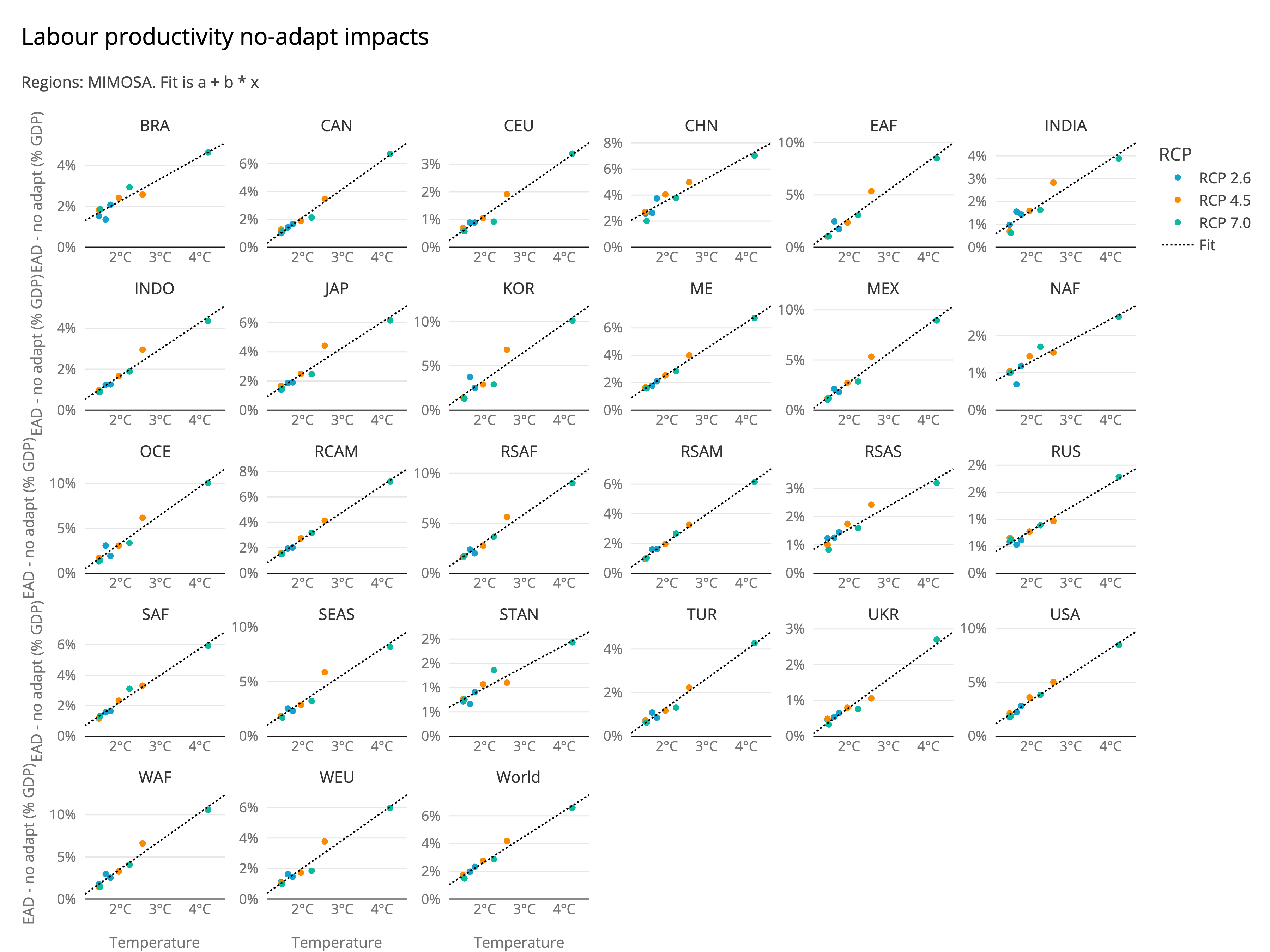
The impact of climate change on labour productivity can be decomposed in two types: heat-related expected annual costs due to warming (e.g. hot regions get hotter, leading to reduced labour productivity), and cold-related expected annual benefits due to less cold days (especially relevant for currently cold regions).

The heat-related gross damage costs are fitted using a linear function of global temperature, shifted to 0 at the start year.

\[ \href{./#var__labourprod_damage_costs_gross}{\text{gross damages}_{\text{labourprod},t,r}} = (\href{./#param__regional.ACCREU.labourprod_noadapt_ead_constant}{a_{r, \text{heat}}} + \href{./#param__regional.ACCREU.labourprod_noadapt_ead_linear}{b_{r, \text{heat}}} \cdot \href{./#var__temperature}{T_t}) - (\href{./#param__regional.ACCREU.labourprod_noadapt_ead_constant}{a_{r, \text{heat}}} + \href{./#param__regional.ACCREU.labourprod_noadapt_ead_linear}{b_{r, \text{heat}}} \cdot \href{./#param__temperature.initial}{T_0}). \]

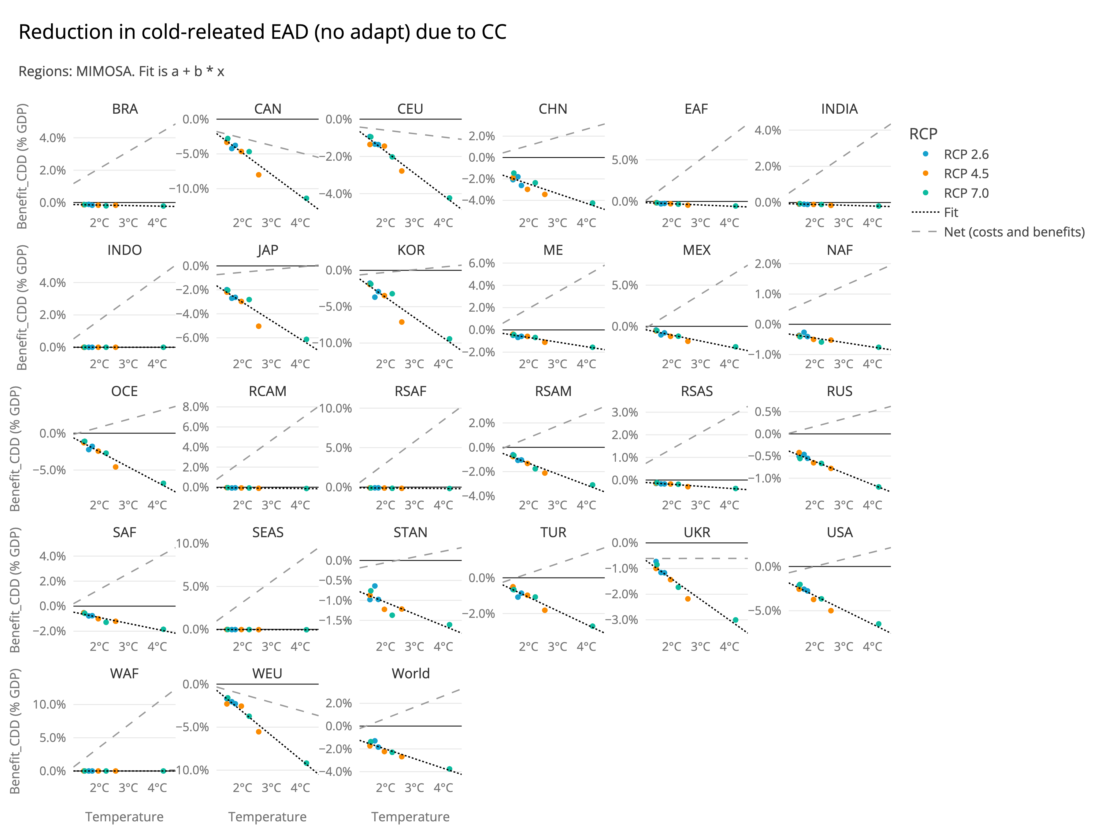
The cold-related benefits of climate change are also fitted using a linear function of global temperature, and shifted to 0 at the start year.

\[ \href{./#var__labourprod_damage_costs_benefits}{\text{benefits}_{\text{labourprod},t,r}} = (\href{./#param__regional.ACCREU.labourprod_benefit_cdd_constant}{a_{r, \text{cold}}} + \href{./#param__regional.ACCREU.labourprod_benefit_cdd_linear}{b_{r, \text{cold}}} \cdot \href{./#var__temperature}{T_t}) - (\href{./#param__regional.ACCREU.labourprod_benefit_cdd_constant}{a_{r, \text{cold}}} + \href{./#param__regional.ACCREU.labourprod_benefit_cdd_linear}{b_{r, \text{cold}}} \cdot \href{./#param__temperature.initial}{T_0}). \]

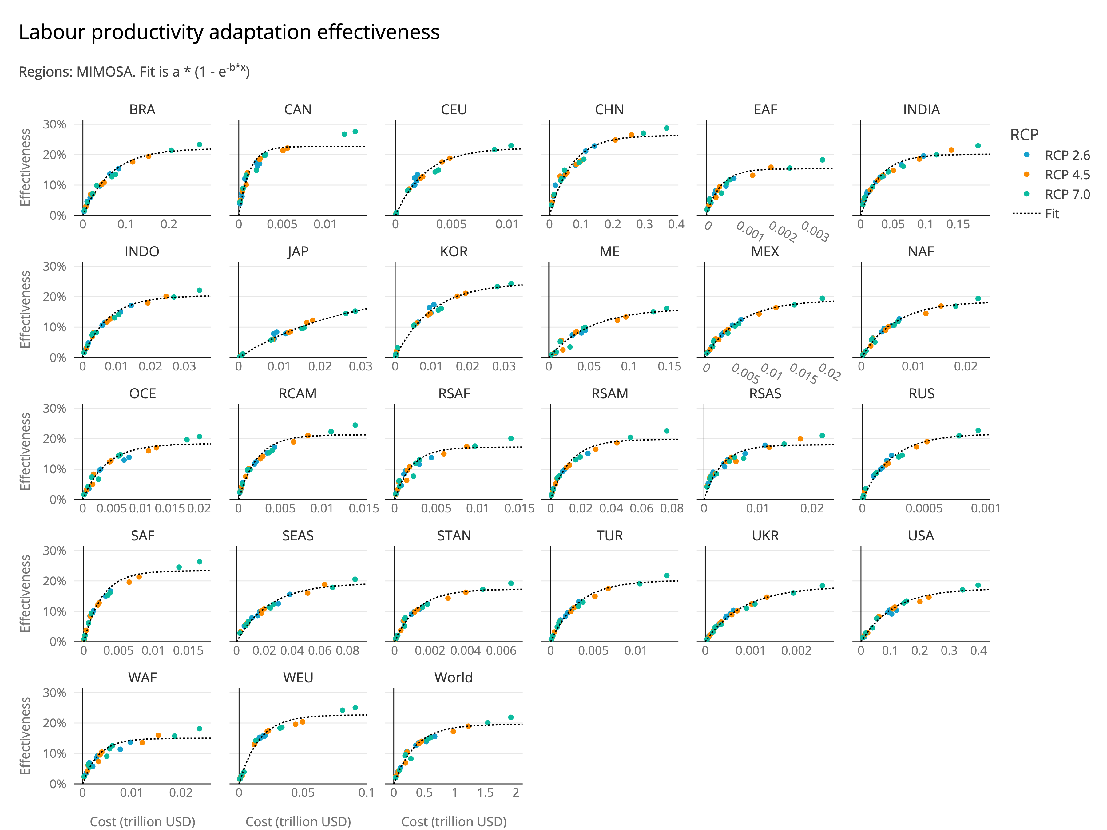
The adaptation function, which only applies to heat-related gross damages, is fitted with a negative-exponential saturation (NES) curve, like in all three sectors, using regional max. effectiveness and cost coefficient:

\[ \href{./#var__labourprod_adaptation_level}{\text{adapt. level}_{\text{labourprod},t,r}} = \text{NES}(\href{./#var__labourprod_adaptation_costs_abs}{\text{adapt. costs}_{\text{labourprod},t,r}}; \href{./#param__regional.ACCREU.labourprod_adapt_eff_max_effectiveness}{\text{max eff.}_{\text{labourprod},r}}, \href{./#param__regional.ACCREU.labourprod_adapt_eff_cost_param}{c_{\text{labourprod},r}}) \]

This leads to the residual, heat related damages:

\[ \href{./#var__labourprod_damage_costs}{\text{damages}_{\text{labourprod},t,r}} = \href{./#var__labourprod_damage_costs_gross}{\text{gross damages}_{\text{labourprod},t,r}} \cdot (1 - \href{./#var__labourprod_adaptation_level}{\text{adapt. level}_{\text{labourprod},t,r}}). \]

The final, net damages are calculated as the sum of the heat-related residual damages and the cold-related benefits:

\[ \href{./#var__labourprod_damage_costs_net}{\text{net damages}_{\text{labourprod},t,r}} = \href{./#var__labourprod_damage_costs}{\text{damages}_{\text{labourprod},t,r}} + \href{./#var__labourprod_damage_costs_benefits}{\text{benefits}_{\text{labourprod},t,r}} \]
  • Global damages (heat- and cold-related, without adapt.)


  • Global adaptation costs (only for heat-related damages)


Regional damage and adaptation functions
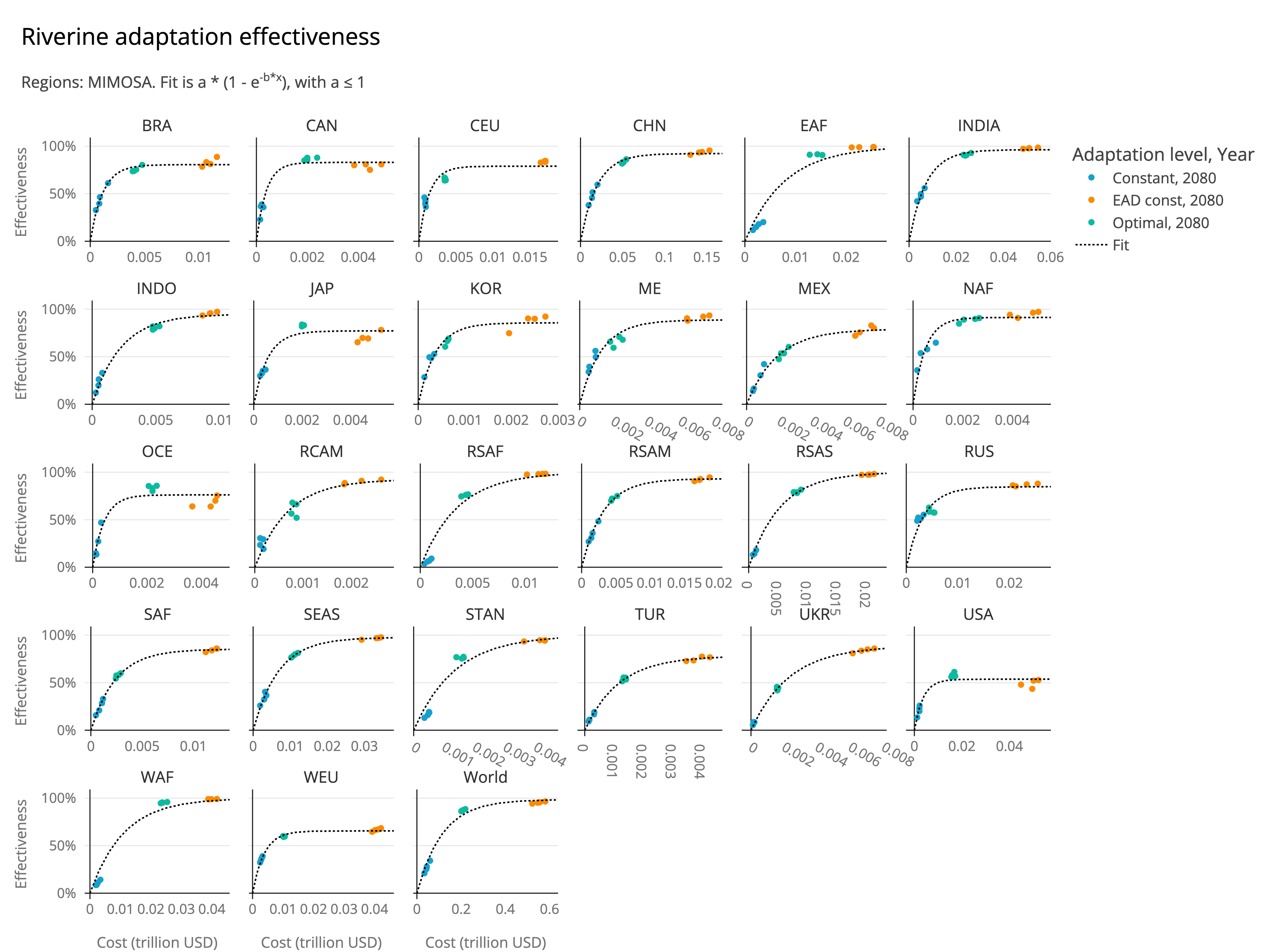
Regional damage costs (without adaptation)

Regional benefits from reduced cold

Regional damage costs (without adaptation)

Variables created in this module:
labourprod_damage_costs_gross: Gross damages from heat-related labour productivity loss (e.g. hot regions get hotter), without adaptation
labourprod_damage_costs_benefits: Benefits from reduced cold days for labour productivity (e.g. cold regions get less cold). No adaptation is applied to these benefits, as they are not related to heat stress.
labourprod_adaptation_costs_abs: Adaptation costs for labour productivity (absolute values) (applied only to heat-related damages, not cold-related benefits)
labourprod_adaptation_costs: Adaptation costs for labour productivity (as a fraction of GDP) (applied only to heat-related damages, not cold-related benefits)
labourprod_adaptation_level: Adaptation level for labour productivity (applied only to heat-related damages, not cold-related benefits)
labourprod_damage_costs: Residual damages for labour productivity after adaptation (heat-related component only)
labourprod_damage_costs_net: Sum of heat-related residual damages and cold-related benefits for labour productivity (net damages)
Source code in mimosa/components/damages/accreu/labour_productivity.py
def get_constraints(
    m: ConcreteModel, inputs: ModelInputs, adaptation_options: AdaptationOptions
):
    r"""

    The impact of climate change on labour productivity can be decomposed in two types:
    heat-related expected annual costs due to warming (e.g. hot regions get hotter, leading
    to reduced labour productivity), and cold-related expected annual benefits due to less cold days
    (especially relevant for currently cold regions).

    :::mimosa.components.damages.accreu.labour_productivity.gross_dmg_fct_labourprod
        options:
            show_source: false

    :::mimosa.components.damages.accreu.labour_productivity.benefits_dmg_fct_labourprod
        options:
            show_source: false

    The adaptation function, which only applies to heat-related gross damages, is fitted with a negative-exponential saturation (NES) curve, like in
    all three sectors, using regional [max. effectiveness](#param__regional.ACCREU.labourprod_adapt_eff_max_effectiveness) and [cost coefficient](#param__regional.ACCREU.labourprod_adapt_eff_cost_param):

    $$
    \href{./#var__labourprod_adaptation_level}{\text{adapt. level}_{\text{labourprod},t,r}}
    = \text{NES}(\href{./#var__labourprod_adaptation_costs_abs}{\text{adapt. costs}_{\text{labourprod},t,r}};
    \href{./#param__regional.ACCREU.labourprod_adapt_eff_max_effectiveness}{\text{max eff.}_{\text{labourprod},r}},
    \href{./#param__regional.ACCREU.labourprod_adapt_eff_cost_param}{c_{\text{labourprod},r}})
    $$

    This leads to the residual, heat related damages:

    $$
    \href{./#var__labourprod_damage_costs}{\text{damages}_{\text{labourprod},t,r}}
    = \href{./#var__labourprod_damage_costs_gross}{\text{gross damages}_{\text{labourprod},t,r}} \cdot (1 - \href{./#var__labourprod_adaptation_level}{\text{adapt. level}_{\text{labourprod},t,r}}).
    $$

    The final, net damages are calculated as the sum of the heat-related residual damages and the cold-related benefits:

    $$
    \href{./#var__labourprod_damage_costs_net}{\text{net damages}_{\text{labourprod},t,r}}
    = \href{./#var__labourprod_damage_costs}{\text{damages}_{\text{labourprod},t,r}}
    + \href{./#var__labourprod_damage_costs_benefits}{\text{benefits}_{\text{labourprod},t,r}}
    $$

    <div class="grid cards" markdown>

    -   <h5 class="no-nav">Global damages (heat- and cold-related, without adapt.)</h5>

        ---

        ``` plotly
        {"file_path": "./assets/plots/labourprod_damages_global.json"}
        ```

    -   <h5 class="no-nav">Global adaptation costs (only for heat-related damages)</h5>

        ---

        ``` plotly
        {"file_path": "./assets/plots/labourprod_adaptation_global.json"}
        ```
    </div>

    ??? regional-fct "Regional damage and adaptation functions"

        === "Damages (without adaptation, heat-related)"

            ![Regional damage costs (without adaptation)](../../assets/fig/accreu/labourprod_noadapt_ead.png)

        === "Benefits (from reduced cold)"

            ![Regional benefits from reduced cold](../../assets/fig/accreu/labourprod_benefit_cdd.png)

        === "Adaptation costs"

            ![Regional damage costs (without adaptation)](../../assets/fig/accreu/labourprod_adapt_eff.png)


    <div class="tiny_table table_scrollable extra_small" markdown>

    | Variables created in this module: |
    | --------------------------------- |
    | var::labourprod_damage_costs_gross |
    | var::labourprod_damage_costs_benefits |
    | var::labourprod_adaptation_costs_abs |
    | var::labourprod_adaptation_costs |
    | var::labourprod_adaptation_level |
    | var::labourprod_damage_costs |
    | var::labourprod_damage_costs_net |

    </div>

    """

    constraints = []

    adaptation_type = adaptation_options.adaptation_type
    adaptation_calibration = adaptation_options.calibrations["labourprod"]

    ## Gross damages:

    damage_cost_gross_var_name = (
        "labourprod_damage_costs"
        if adaptation_type == "noadaptation"
        else "labourprod_damage_costs_gross"
    )

    setattr(
        m,
        damage_cost_gross_var_name,
        Var(
            m.t,
            m.regions,
            units=quant.unit("fraction_of_GDP"),
            doc="Gross damages from heat-related labour productivity loss (e.g. hot regions get hotter), without adaptation",
        ),
    )

    m.labourprod_damages_gross_constant = Param(
        m.regions,
        initialize=inputs.regional("ACCREU", "labourprod_noadapt_ead_constant"),
    )
    m.labourprod_damages_gross_linear = Param(
        m.regions, initialize=inputs.regional("ACCREU", "labourprod_noadapt_ead_linear")
    )

    constraints.append(
        RegionalEquation(
            getattr(m, damage_cost_gross_var_name), gross_dmg_fct_labourprod
        )
    )

    ## Benefits from less cooling demand due to higher temperatures (negative damages):

    m.labourprod_damage_costs_benefits = Var(
        m.t,
        m.regions,
        units=quant.unit("fraction_of_GDP"),
        doc="Benefits from reduced cold days for labour productivity (e.g. cold regions get less cold). No adaptation is applied to these benefits, as they are not related to heat stress.",
    )

    m.labourprod_damages_benefits_constant = Param(
        m.regions,
        initialize=inputs.regional("ACCREU", "labourprod_benefit_cdd_constant"),
    )
    m.labourprod_damages_benefits_linear = Param(
        m.regions, initialize=inputs.regional("ACCREU", "labourprod_benefit_cdd_linear")
    )

    constraints.append(
        RegionalEquation(
            m.labourprod_damage_costs_benefits, benefits_dmg_fct_labourprod
        )
    )

    ## Adaptation (only for costs, doesn't apply to benefits):

    if adaptation_type == "sectoral":
        m.labourprod_adaptation_costs_abs = Var(
            m.t,
            m.regions,
            units=quant.unit("currency_unit"),
            doc="Adaptation costs for labour productivity (absolute values) (applied only to heat-related damages, not cold-related benefits)",
            bounds=lambda m, t, r: (0, 0.1 * m.baseline_GDP[t, r]),
        )
        m.labourprod_adaptation_costs = Var(
            m.t,
            m.regions,
            units=quant.unit("fraction_of_GDP"),
            doc="Adaptation costs for labour productivity (as a fraction of GDP) (applied only to heat-related damages, not cold-related benefits)",
        )
        m.labourprod_adaptation_level = Var(
            m.t,
            m.regions,
            units=quant.unit("fraction_of_gross_damages"),
            bounds=(0, 1),
            doc="Adaptation level for labour productivity (applied only to heat-related damages, not cold-related benefits)",
        )
        m.labourprod_damage_costs = Var(
            m.t,
            m.regions,
            units=quant.unit("fraction_of_GDP"),
            doc="Residual damages for labour productivity after adaptation (heat-related component only)",
        )

        m.labourprod_adaptation_max_effectiveness = Param(
            m.regions,
            initialize=inputs.regional(
                "ACCREU", "labourprod_adapt_eff_max_effectiveness"
            ),
        )
        m.labourprod_adaptation_cost_param = Param(
            m.regions,
            initialize=inputs.regional("ACCREU", "labourprod_adapt_eff_cost_param"),
        )
        constraints.append(
            get_delayed_adaptation_constraint("labourprod_adaptation_costs")
        )
        constraints.extend(
            [
                # Adaptation effectiveness function
                RegionalEquation(
                    m.labourprod_adaptation_level,
                    lambda m, t, r: adaptation_effectiveness_fct(
                        m.labourprod_adaptation_costs_abs[t, r],
                        *effective_adaptation_curve(
                            m,
                            r,
                            m.labourprod_adaptation_max_effectiveness[r],
                            m.labourprod_adaptation_cost_param[r],
                            adaptation_calibration,
                        ),
                    ),
                ),
                # Adaptation costs as a fraction of GDP
                RegionalEquation(
                    m.labourprod_adaptation_costs,
                    lambda m, t, r: m.labourprod_adaptation_costs_abs[t, r]
                    / m.GDP_gross[t, r],
                ),
                # Residual damages after adaptation
                RegionalEquation(
                    m.labourprod_damage_costs,
                    lambda m, t, r: m.labourprod_damage_costs_gross[t, r]
                    * (1 - m.labourprod_adaptation_level[t, r]),
                ),
            ]
        )

        if adaptation_options.uses_analytical_adaptation:
            constraints.append(
                # Calculate analytically the optimal level of adaptation
                RegionalEquation(
                    m.labourprod_adaptation_costs_abs,
                    lambda m, t, r: optimal_adaptation_costs_fct(
                        m,
                        t,
                        m.labourprod_damage_costs_gross[t, r] * m.GDP_gross[t, r],
                        *effective_adaptation_curve(
                            m,
                            r,
                            m.labourprod_adaptation_max_effectiveness[r],
                            m.labourprod_adaptation_cost_param[r],
                            adaptation_calibration,
                        ),
                    ),
                )
            )

    if adaptation_type != "combined":
        ## Net damages (costs + negative benefits):

        m.labourprod_damage_costs_net = Var(
            m.t,
            m.regions,
            units=quant.unit("fraction_of_GDP"),
            doc="Sum of heat-related residual damages and cold-related benefits for labour productivity (net damages)",
        )

        constraints.append(
            RegionalEquation(
                m.labourprod_damage_costs_net,
                lambda m, t, r: m.labourprod_damage_costs[t, r]
                + m.labourprod_damage_costs_benefits[t, r],
            )
        )

    return constraints

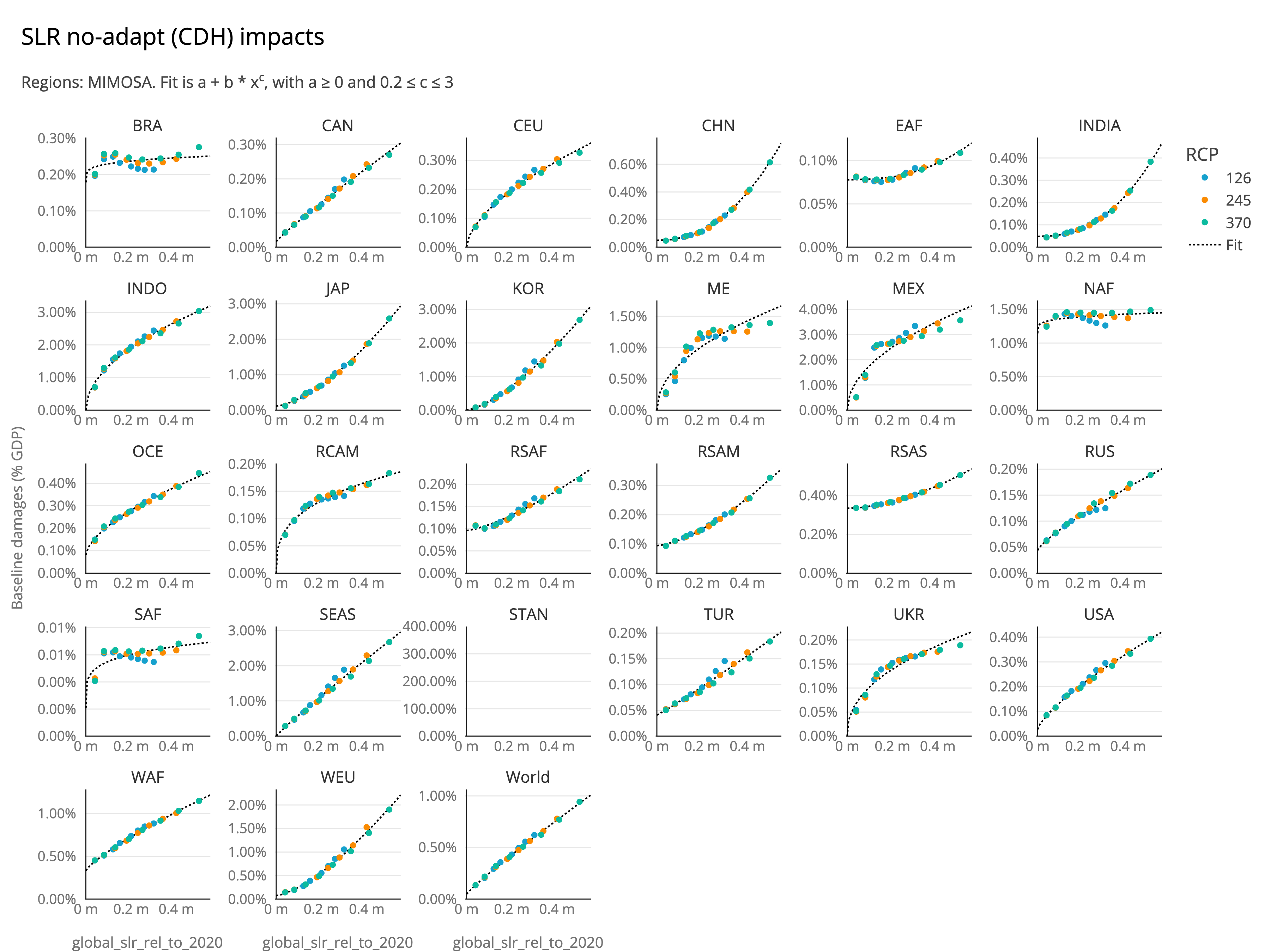
The sea-level rise impacts are calculated using the DIVA model. Specifically, for this purpose, we compare the Constant Dike Height scenario (“no adaptation / CDH”) with three adaptation scenarios: Constant flood protection standards, Doubling flood protection standards, and Quadrupling flood protection standards. Importantly, we do not use the “optimal adaptation” scenario from DIVA, to avoid double optimisation in the IAMs.

The gross damages are fitted with a power function of global sea-level rise:

\[ \href{./#var__slr_damage_costs_gross}{\text{gross damages}_{\text{SLR},t,r}} = \left(\href{./#param__regional.ACCREU.slr_noadapt_ead_constant}{a_r} + \href{./#param__regional.ACCREU.slr_noadapt_ead_prod}{b_r} \cdot \left(\href{./#var__total_SLR}{\text{SLR}_t}\right)^{\href{./#param__regional.ACCREU.slr_noadapt_ead_power}{c_r}}\right) - \left(\href{./#param__regional.ACCREU.slr_noadapt_ead_constant}{a_r} + \href{./#param__regional.ACCREU.slr_noadapt_ead_prod}{b_r} \cdot \left(\href{./#var__total_SLR}{\text{SLR}_0}\right)^{\href{./#param__regional.ACCREU.slr_noadapt_ead_power}{c_r}}\right) \]

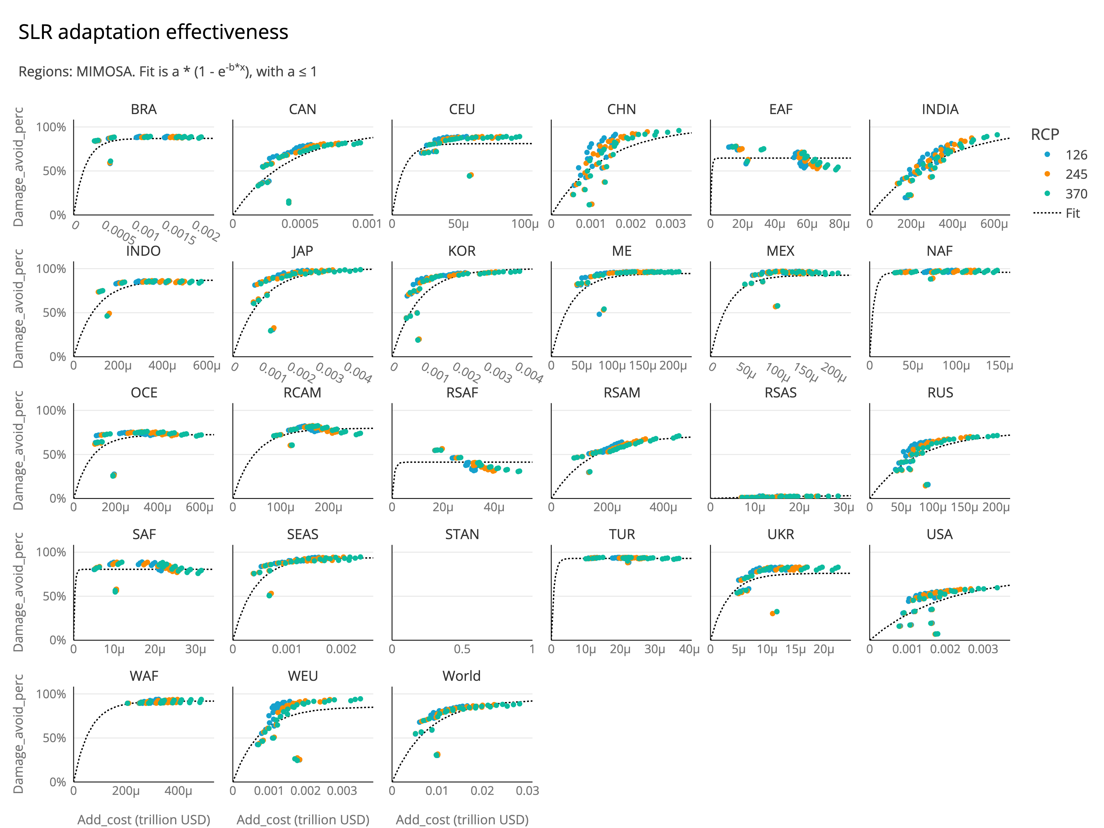
The adaptation function is fitted with a negative-exponential saturation (NES) curve, like in all three sectors, using regional max. effectiveness and cost coefficient:

\[ \href{./#var__slr_adaptation_level}{\text{adapt. level}_{\text{SLR},t,r}} = \text{NES}(\href{./#var__slr_adaptation_costs_abs}{\text{adapt. costs}_{\text{SLR},t,r}}; \href{./#param__regional.ACCREU.slr_adapt_eff_max_effectiveness}{\text{max eff.}_{\text{SLR},r}}, \href{./#param__regional.ACCREU.slr_adapt_eff_cost_param}{c_{\text{SLR},r}}) \]

Subsequently, the residual damages are calculated as:

\[ \href{./#var__slr_damage_costs}{\text{damages}_{\text{SLR},t,r}} = \href{./#var__slr_damage_costs_gross}{\text{gross damages}_{\text{SLR},t,r}} \cdot (1 - \href{./#var__slr_adaptation_level}{\text{adapt. level}_{\text{SLR},t,r}}), \]
  • Global damages (without adaptation)


  • Global adaptation costs


Regional damage and adaptation functions
Regional damage costs (without adaptation)

Regional damage costs (without adaptation)

Variables created in this module:
slr_damage_costs_gross: Gross damages from sea-level rise, without adaptation
slr_adaptation_costs_abs: Absolute adaptation costs for sea-level rise, in currency units. Used to calculate the adaptation level
slr_adaptation_costs: Adaptation costs for sea-level rise, as a fraction of GDP.
slr_adaptation_level: Adaptation level for sea-level rise, as a fraction of gross damages. 0 means that no damages are avoided, while 1 means that all damages are avoided.
slr_damage_costs: Residual damages from sea-level rise, after adaptation. If `noadaptation` is chosen, this variable represents the gross damages.
Source code in mimosa/components/damages/accreu/sealevelrise.py
def get_constraints(
    m: ConcreteModel, inputs: ModelInputs, adaptation_options: AdaptationOptions
):
    r"""

    The sea-level rise impacts are calculated using the DIVA model. Specifically,
    for this purpose, we compare the Constant Dike Height scenario (“no adaptation / CDH”)
    with three adaptation scenarios: Constant flood protection standards, Doubling
    flood protection standards, and Quadrupling flood protection standards. Importantly,
    we do not use the “optimal adaptation” scenario from DIVA, to avoid double optimisation
    in the IAMs.

    The gross damages are fitted with a power function of global sea-level rise:

    :::mimosa.components.damages.accreu.sealevelrise.gross_dmg_fct_slr
        options:
            show_source: false

    The adaptation function is fitted with a negative-exponential saturation (NES) curve, like in
    all three sectors, using regional [max. effectiveness](#param__regional.ACCREU.slr_adapt_eff_max_effectiveness) and [cost coefficient](#param__regional.ACCREU.slr_adapt_eff_cost_param):

    $$
    \href{./#var__slr_adaptation_level}{\text{adapt. level}_{\text{SLR},t,r}}
    = \text{NES}(\href{./#var__slr_adaptation_costs_abs}{\text{adapt. costs}_{\text{SLR},t,r}};
    \href{./#param__regional.ACCREU.slr_adapt_eff_max_effectiveness}{\text{max eff.}_{\text{SLR},r}},
    \href{./#param__regional.ACCREU.slr_adapt_eff_cost_param}{c_{\text{SLR},r}})
    $$

    Subsequently, the residual damages are calculated as:

    $$
    \href{./#var__slr_damage_costs}{\text{damages}_{\text{SLR},t,r}} = \href{./#var__slr_damage_costs_gross}{\text{gross damages}_{\text{SLR},t,r}} \cdot (1 - \href{./#var__slr_adaptation_level}{\text{adapt. level}_{\text{SLR},t,r}}),
    $$

    <div class="grid cards" markdown>

    -   <h5 class="no-nav">Global damages (without adaptation)</h5>

        ---

        ``` plotly
        {"file_path": "./assets/plots/slr_damages_global.json"}
        ```

    -   <h5 class="no-nav">Global adaptation costs</h5>

        ---

        ``` plotly
        {"file_path": "./assets/plots/slr_adaptation_global.json"}
        ```
    </div>

    ??? regional-fct "Regional damage and adaptation functions"

        === "Damages (without adaptation)"

            ![Regional damage costs (without adaptation)](../../assets/fig/accreu/slr_noadapt_ead.png)

        === "Adaptation costs"

            ![Regional damage costs (without adaptation)](../../assets/fig/accreu/slr_adapt_eff.png)

    <div class="tiny_table table_scrollable extra_small" markdown>

    | Variables created in this module: |
    | --------------------------------- |
    | var::slr_damage_costs_gross |
    | var::slr_adaptation_costs_abs |
    | var::slr_adaptation_costs |
    | var::slr_adaptation_level |
    | var::slr_damage_costs |

    </div>
    """

    constraints = []
    adaptation_type = adaptation_options.adaptation_type
    adaptation_calibration = adaptation_options.calibrations["slr"]

    ## Gross damages:

    m.slr_damages_gross_constant = Param(
        m.regions, initialize=inputs.regional("ACCREU", "slr_noadapt_ead_constant")
    )
    m.slr_damages_gross_prod = Param(
        m.regions, initialize=inputs.regional("ACCREU", "slr_noadapt_ead_prod")
    )
    m.slr_damages_gross_power = Param(
        m.regions, initialize=inputs.regional("ACCREU", "slr_noadapt_ead_power")
    )

    damage_cost_gross_var_name = (
        "slr_damage_costs"
        if adaptation_type == "noadaptation"
        else "slr_damage_costs_gross"
    )
    setattr(
        m,
        damage_cost_gross_var_name,
        Var(
            m.t,
            m.regions,
            units=quant.unit("fraction_of_GDP"),
            doc="Gross damages from sea-level rise, without adaptation",
        ),
    )
    constraints.append(
        RegionalEquation(
            getattr(m, damage_cost_gross_var_name),
            gross_dmg_fct_slr,
        )
    )

    ## Adaptation:
    if adaptation_type != "noadaptation":
        m.slr_adaptation_costs_abs = Var(
            m.t,
            m.regions,
            units=quant.unit("currency_unit"),
            bounds=lambda m, t, r: (0, 0.1 * m.baseline_GDP[t, r]),
            doc="Absolute adaptation costs for sea-level rise, in currency units. Used to calculate the adaptation level",
        )
        m.slr_adaptation_costs = Var(
            m.t,
            m.regions,
            units=quant.unit("fraction_of_GDP"),
            doc="Adaptation costs for sea-level rise, as a fraction of GDP.",
        )
        m.slr_adaptation_level = Var(
            m.t,
            m.regions,
            units=quant.unit("fraction_of_gross_damages"),
            bounds=(0, 1),
            doc="Adaptation level for sea-level rise, as a fraction of gross damages. 0 means that no damages are avoided, while 1 means that all damages are avoided.",
        )
        m.slr_damage_costs = Var(
            m.t,
            m.regions,
            units=quant.unit("fraction_of_GDP"),
            doc="Residual damages from sea-level rise, after adaptation. If `noadaptation` is chosen, this variable represents the gross damages.",
        )

        m.slr_adaptation_max_effectiveness = Param(
            m.regions,
            initialize=inputs.regional("ACCREU", "slr_adapt_eff_max_effectiveness"),
        )
        m.slr_adaptation_cost_param = Param(
            m.regions,
            initialize=inputs.regional("ACCREU", "slr_adapt_eff_cost_param"),
        )
        constraints.append(get_delayed_adaptation_constraint("slr_adaptation_costs"))
        constraints.extend(
            [
                # Adaptation effectiveness function
                RegionalEquation(
                    m.slr_adaptation_level,
                    lambda m, t, r: adaptation_effectiveness_fct(
                        m.slr_adaptation_costs_abs[t, r],
                        *effective_adaptation_curve(
                            m,
                            r,
                            m.slr_adaptation_max_effectiveness[r],
                            m.slr_adaptation_cost_param[r],
                            adaptation_calibration,
                        ),
                    ),
                ),
                # Adaptation costs as a fraction of GDP
                RegionalEquation(
                    m.slr_adaptation_costs,
                    lambda m, t, r: m.slr_adaptation_costs_abs[t, r]
                    / m.GDP_gross[t, r],
                ),
                # Residual damages after adaptation
                RegionalEquation(
                    m.slr_damage_costs,
                    lambda m, t, r: m.slr_damage_costs_gross[t, r]
                    * (1 - m.slr_adaptation_level[t, r]),
                ),
            ]
        )

        if adaptation_options.uses_analytical_adaptation:
            constraints.append(
                # Calculate analytically the optimal level of adaptation
                RegionalEquation(
                    m.slr_adaptation_costs_abs,
                    lambda m, t, r: optimal_adaptation_costs_fct(
                        m,
                        t,
                        m.slr_damage_costs_gross[t, r] * m.GDP_gross[t, r],
                        *effective_adaptation_curve(
                            m,
                            r,
                            m.slr_adaptation_max_effectiveness[r],
                            m.slr_adaptation_cost_param[r],
                            adaptation_calibration,
                        ),
                        scale=0.00001,
                    ),
                )
            )

    return constraints

Physical impacts

The ACCREU damage representation includes temperature-related mortality impacts, though without accounting for explicit adaptation. Like labour productivity, there is a heat-related and cold-related component, varying strongly between regions. As global mean temperature increases, the heat-related mortality increases, while the cold-related mortality decreases.

The mortality forecasts are sourced from Bressler et al. (2021). The paper forecasts the change in future heat-related and cold-related mortality rates under RCP 2.6, RCP 4.5, RCP 6.0 and RCP 8.5 scenarios. It does so for the 2040-59 and 2080-99 periods. For this analysis, the estimates for these ranges are assigned to the years 2050 and 2090 respectively. In order to convert the forecasted change in the mortality rate into an estimate of excess mortality, the Bressler forecasts were combined with mortality rate forecasts from the World Bank (2025).

The heat-related mortality (as % of population) was fitted with a quadratic function. Given that they represent additional mortality relative to 2010, the fit was relative to temperature in 2010: 1.1 °C. To obtain a mortality value in absolute numbers, we multiply by total population:

\[ \href{./#var__mortality_heat_related}{\text{mortality}_{\text{heat}, t, r}} = \href{./#param__timeandregional.population}{\text{population}_{t,r}} \cdot {\large(} (\href{./#param__regional.ACCREU.heat_related_mortality_perc_constant}{a_r} + \href{./#param__regional.ACCREU.heat_related_mortality_perc_prod}{b_r} \cdot (\href{./#var__temperature}{T_t} - 1.1)^2) - (\href{./#param__regional.ACCREU.heat_related_mortality_perc_constant}{a_r} + \href{./#param__regional.ACCREU.heat_related_mortality_perc_prod}{b_r} \cdot (\href{./#var__temperature}{T_0} - 1.1)^2) {\large)} \]

Cold-related mortality showed a linear relation with temperature, accounting for the fact that reductions in cold-related mortality don't become marginally larger when temperatures become very high. In fact, at some point we expect to see a plateau. However, the data doesn't show this behaviour for the assessed temperature range, where a linear fit throughout is the best fit:

\[ \href{./#var__mortality_cold_related}{\text{mortality}_{\text{cold}, t, r}} = \href{./#param__timeandregional.population}{\text{population}_{t,r}} \cdot {\large(} (\href{./#param__regional.ACCREU.cold_related_mortality_perc_constant}{a_r} + \href{./#param__regional.ACCREU.cold_related_mortality_perc_prod}{b_r} \cdot (\href{./#var__temperature}{T_t} - 1.1)) - (\href{./#param__regional.ACCREU.cold_related_mortality_perc_constant}{a_r} + \href{./#param__regional.ACCREU.cold_related_mortality_perc_prod}{b_r} \cdot (\href{./#var__temperature}{T_0} - 1.1)) {\large)} \]

The total mortality is the sum of both:

\[ \href{./#var__mortality_net}{\text{mortality}_{\text{net},t,r}} = \href{./#var__mortality_heat_related}{\text{mortality}_{\text{heat}, t, r}} + \href{./#var__mortality_cold_related}{\text{mortality}_{\text{cold}, t, r}}. \]
  • Global mortality (heat- and cold-related, without adaptation)


Variables created in this module:
mortality_heat_related: Extra heat-related mortality, in absolute numbers. Extra is compared to start year of the run (2025).
mortality_cold_related: Reduced cold-related mortality, in absolute numbers, compared to start year of the run (2025).
mortality_net: Sum of extra heat-related mortality and reduced cold-related mortality, in absolute numbers.

Monetisation of mortality

If the MIMOSA parameter monetise mortality is set to true, the mortality values are converted to monetary value, which are then used by the welfare function:

params = load_params()
params["economics"]["damages"]["accreu"]["monetise_mortality"] = True # or False
model = MIMOSA(params)

Valuation of mortality in monetary units can be done using values of statistical life (VSL) or values of statistical life years (VSLY) multiplied by the expected life years lost. The main difference between these valuation methods is that the VSLY approach gives relatively lower values to mortality of people with a lower remaining life expectancy, while the VSL approach values mortality in all age classes equally.

Here, we follow the recommendation by the OECD to not adjust valuation according to the age of the population as this would imply that public policy and cost-benefit analysis outcomes could differ solely based on differences in the age of the populations studied. Moreover, little is known about the expected life years lost due to climate change impacts (Toulemon & Barbieri, 2008).

We therefore use the VSL approach for valuing the cost of mortality. The default MIMOSA value is the recommended estimates of the VSL from the OECD (2025). They provide a weighted world value of the VSL of 2.4 million dollars, which gives a \(\text{VSL}_{\text{rel}}\) of 117.59 times the GDP per capita.

The VSL in dollar terms is therefore:

\[ \href{./#var__mortality_vsl}{\text{VSL}_{\text{abs},t,r}} = \href{./#param__economics.damages.accreu.mortality_vsl_rel_gdp_cap}{\text{VSL}_{\text{rel}}} \cdot \frac{\href{./#var__GDP_gross}{\text{GDP}_{\text{gross},t,r}}}{\href{./#param__timeandregional.population}{\text{population}_{t,r}}} \]

The resulting mortality costs (in absolute terms) are given by:

\[ \begin{align} \href{./#var__mortality_damage_costs_abs}{\text{abs. damages}_{\text{mortality}, t, r}} &=\href{./#var__mortality_vsl}{\text{VSL}_{\text{abs},t,r}} \cdot (\href{./#var__mortality_heat_related}{\text{mortality}_{\text{heat}, t, r}} + \href{./#var__mortality_cold_related}{\text{mortality}_{\text{cold}, t, r}})\\ &= \href{./#var__non_market_damage_costs_abs}{\text{abs. damages}_{\text{non-market}, t,r}} \end{align} \]

Since these are the only non-market damages in the model, the non-market damages are equal to the mortality costs. These are not subtracted from GDP, but are removed in the welfare function. damages.

Variables created when mortality is monetised:
mortality_vsl: Value of statistical life (VSL) in currency units, calculated as the relative VSL times GDP per capita
mortality_damage_costs_abs: Mortality damage costs in currency units. Since the extra heat-related deaths and reduced cold-related deaths are considered, this value can be positive or negative, depending on the region, time, and temperature.
mortality_damage_costs: Mortality damage costs expressed as % of GDP
Source code in mimosa/components/damages/accreu/mortality.py
def _get_monetised_mortality_constraints(m: ConcreteModel, inputs: ModelInputs):
    r"""
    If the MIMOSA parameter [monetise mortality](#param__economics.damages.accreu.monetise_mortality)
    is set to true, the mortality values are converted to monetary value, which are then used
    by the welfare function:

    ```python hl_lines="2"
    params = load_params()
    params["economics"]["damages"]["accreu"]["monetise_mortality"] = True # or False
    model = MIMOSA(params)
    ```

    Valuation of mortality in monetary units can be done using values of
    statistical life (VSL) or values of statistical life years (VSLY) multiplied by the expected
    life years lost. The main difference between these valuation methods is that the
    VSLY approach gives relatively lower values to mortality of people with a lower
    remaining life expectancy, while the VSL approach values mortality in all age
    classes equally.

    Here, we follow the recommendation by the OECD to not adjust valuation according
    to the age of the population as this would imply that public policy and cost-benefit
    analysis outcomes could differ solely based on differences in the age of the populations
    studied. Moreover, little is known about the expected life years lost due to climate
    change impacts (Toulemon & Barbieri, 2008).

    We therefore use the VSL approach for valuing the cost of mortality. The default MIMOSA
    value is the recommended estimates of the VSL from the OECD (2025). They provide a weighted
    world value of the VSL of 2.4 million dollars, which gives a [$\text{VSL}_{\text{rel}}$](#param__economics.damages.accreu.mortality_vsl_rel_gdp_cap)
    of 117.59 times the GDP per capita.

    The VSL in dollar terms is therefore:

    $$
    \href{./#var__mortality_vsl}{\text{VSL}_{\text{abs},t,r}}
    = \href{./#param__economics.damages.accreu.mortality_vsl_rel_gdp_cap}{\text{VSL}_{\text{rel}}}
    \cdot \frac{\href{./#var__GDP_gross}{\text{GDP}_{\text{gross},t,r}}}{\href{./#param__timeandregional.population}{\text{population}_{t,r}}}
    $$


    The resulting mortality costs (in absolute terms) are given by:

    $$
    \begin{align}
        \href{./#var__mortality_damage_costs_abs}{\text{abs. damages}_{\text{mortality}, t, r}}
        &=\href{./#var__mortality_vsl}{\text{VSL}_{\text{abs},t,r}} \cdot (\href{./#var__mortality_heat_related}{\text{mortality}_{\text{heat}, t, r}}
        + \href{./#var__mortality_cold_related}{\text{mortality}_{\text{cold}, t, r}})\\
        &= \href{./#var__non_market_damage_costs_abs}{\text{abs. damages}_{\text{non-market}, t,r}}
    \end{align}
    $$

    Since these are the only non-market damages in the model, the non-market damages are equal to the
    mortality costs. These are not subtracted from GDP, but are removed in the [welfare function](../welfare.md).
    damages. 

    <div class="tiny_table table_scrollable extra_small" markdown>

    | Variables created when mortality is monetised: |
    | --------------------------------- |
    | var::mortality_vsl |
    | var::mortality_damage_costs_abs |
    | var::mortality_damage_costs |

    </div>

    """

    # Calculate the monetary damages from mortality, using the value of a statistical life (VSL)
    m.mortality_vsl_rel_gdp_per_cap = Param(
        initialize=inputs.config("economics.damages.accreu.mortality_vsl_rel_gdp_cap")
    )

    m.mortality_vsl = Var(
        m.t,
        m.regions,
        units=quant.unit("currency_unit"),
        doc="Value of statistical life (VSL) in currency units, calculated as the relative VSL times GDP per capita",
    )
    m.mortality_damage_costs_abs = Var(
        m.t,
        m.regions,
        units=quant.unit("currency_unit"),
        bounds=lambda m, t, r: (
            -0.1 * m.baseline_GDP[t, r],
            0.5 * m.baseline_GDP[t, r],
        ),
        doc="Mortality damage costs in currency units. Since the extra heat-related deaths and reduced cold-related deaths are considered, this value can be positive or negative, depending on the region, time, and temperature.",
    )
    m.mortality_damage_costs = Var(
        m.t,
        m.regions,
        units=quant.unit("fraction_of_GDP"),
        doc="Mortality damage costs expressed as % of GDP",
    )
    constraints = [
        RegionalEquation(
            m.mortality_vsl,
            lambda m, t, r: m.mortality_vsl_rel_gdp_per_cap
            * m.GDP_gross[t, r]
            / m.population[t, r],
        ),
        RegionalEquation(
            m.mortality_damage_costs_abs,
            lambda m, t, r: m.mortality_vsl[t, r]
            * (m.mortality_cold_related[t, r] + m.mortality_heat_related[t, r]),
        ),
        RegionalEquation(
            m.mortality_damage_costs,
            lambda m, t, r: m.mortality_damage_costs_abs[t, r] / m.GDP_gross[t, r],
        ),
    ]

    return constraints
Source code in mimosa/components/damages/accreu/mortality.py
def get_constraints(m: ConcreteModel, inputs: ModelInputs, monetise_mortality=False):
    r"""

    ### Physical impacts

    The ACCREU damage representation includes temperature-related mortality impacts, though
    without accounting for explicit adaptation. Like labour productivity, there is a heat-related
    and cold-related component, varying strongly between regions. As global mean temperature increases,
    the heat-related mortality increases, while the cold-related mortality decreases.

    The mortality forecasts are sourced from Bressler et al. (2021). The paper forecasts the change in
    future heat-related and cold-related mortality rates under RCP 2.6, RCP 4.5, RCP 6.0 and RCP 8.5 scenarios.
    It does so for the 2040-59 and 2080-99 periods. For this analysis, the estimates for these ranges are assigned
    to the years 2050 and 2090 respectively. In order to convert the forecasted change in the mortality rate
    into an estimate of excess mortality, the Bressler forecasts were combined with mortality rate forecasts
    from the World Bank (2025).

    The heat-related mortality (as % of population) was fitted with a quadratic function. Given that they represent
    additional mortality relative to 2010, the fit was relative to temperature in 2010: 1.1 °C. To obtain a mortality
    value in absolute numbers, we multiply by total population:

    $$
    \href{./#var__mortality_heat_related}{\text{mortality}_{\text{heat}, t, r}}
    = \href{./#param__timeandregional.population}{\text{population}_{t,r}}
    \cdot {\large(}
        (\href{./#param__regional.ACCREU.heat_related_mortality_perc_constant}{a_r}
        + \href{./#param__regional.ACCREU.heat_related_mortality_perc_prod}{b_r}
        \cdot (\href{./#var__temperature}{T_t} - 1.1)^2)
        - (\href{./#param__regional.ACCREU.heat_related_mortality_perc_constant}{a_r}
        + \href{./#param__regional.ACCREU.heat_related_mortality_perc_prod}{b_r}
        \cdot (\href{./#var__temperature}{T_0} - 1.1)^2)
    {\large)}
    $$

    Cold-related mortality showed a linear relation with temperature, accounting for the fact that reductions in
    cold-related mortality don't become marginally larger when temperatures become very high. In fact, at some point
    we expect to see a plateau. However, the data doesn't show this behaviour for the assessed temperature range, where
    a linear fit throughout is the best fit:

    $$
    \href{./#var__mortality_cold_related}{\text{mortality}_{\text{cold}, t, r}}
    = \href{./#param__timeandregional.population}{\text{population}_{t,r}}
    \cdot {\large(}
        (\href{./#param__regional.ACCREU.cold_related_mortality_perc_constant}{a_r}
        + \href{./#param__regional.ACCREU.cold_related_mortality_perc_prod}{b_r}
        \cdot (\href{./#var__temperature}{T_t} - 1.1))
        - (\href{./#param__regional.ACCREU.cold_related_mortality_perc_constant}{a_r}
        + \href{./#param__regional.ACCREU.cold_related_mortality_perc_prod}{b_r}
        \cdot (\href{./#var__temperature}{T_0} - 1.1))
    {\large)}
    $$

    The total mortality is the sum of both:

    $$
    \href{./#var__mortality_net}{\text{mortality}_{\text{net},t,r}}
    = \href{./#var__mortality_heat_related}{\text{mortality}_{\text{heat}, t, r}}
    + \href{./#var__mortality_cold_related}{\text{mortality}_{\text{cold}, t, r}}.
    $$


    <div class="grid cards" markdown>

    -   <h5 class="no-nav">Global mortality (heat- and cold-related, without adaptation)</h5>

        ---

        ``` plotly
        {"file_path": "./assets/plots/mortality_global.json"}
        ```
    </div>

    <div class="tiny_table table_scrollable extra_small" markdown>

    | Variables created in this module: |
    | --------------------------------- |
    | var::mortality_heat_related |
    | var::mortality_cold_related |
    | var::mortality_net |

    </div>

    ### Monetisation of mortality

    :::mimosa.components.damages.accreu.mortality._get_monetised_mortality_constraints

    """

    constraints = []

    ## Heat related mortality:
    m.mortality_heat_related = Var(
        m.t,
        m.regions,
        units=quant.unit("billion people"),
        doc="Extra heat-related mortality, in absolute numbers. Extra is compared to start year of the run (2025).",
    )

    m.mortality_heat_related_constant = Param(
        m.regions,
        initialize=inputs.regional("ACCREU", "heat_related_mortality_perc_constant"),
    )
    m.mortality_heat_related_prod = Param(
        m.regions,
        initialize=inputs.regional("ACCREU", "heat_related_mortality_perc_prod"),
    )

    constraints.append(
        RegionalEquation(
            m.mortality_heat_related,
            lambda m, t, r: m.population[t, r]
            * dmg_fct_power(
                m,
                t,
                m.mortality_heat_related_constant[r],
                m.mortality_heat_related_prod[r],
                2,
                xshift=1.1,
            ),
        )
    )

    ## Cold related mortality:
    m.mortality_cold_related = Var(
        m.t,
        m.regions,
        units=quant.unit("billion people"),
        doc="Reduced cold-related mortality, in absolute numbers, compared to start year of the run (2025).",
    )

    m.mortality_cold_related_constant = Param(
        m.regions,
        initialize=inputs.regional("ACCREU", "cold_related_mortality_perc_constant"),
    )
    m.mortality_cold_related_prod = Param(
        m.regions,
        initialize=inputs.regional("ACCREU", "cold_related_mortality_perc_prod"),
    )

    constraints.append(
        RegionalEquation(
            m.mortality_cold_related,
            lambda m, t, r: m.population[t, r]
            * dmg_fct_linear(
                m,
                t,
                m.mortality_cold_related_constant[r],
                m.mortality_cold_related_prod[r],
                xshift=1.1,
            ),
        )
    )

    ## Net mortality (heat + cold related):
    m.mortality_net = Var(
        m.t,
        m.regions,
        units=quant.unit("billion people"),
        doc="Sum of extra heat-related mortality and reduced cold-related mortality, in absolute numbers.",
    )
    constraints.append(
        RegionalEquation(
            m.mortality_net,
            lambda m, t, r: m.mortality_cold_related[t, r]
            + m.mortality_heat_related[t, r],
        )
    )

    if monetise_mortality:
        constraints.extend(_get_monetised_mortality_constraints(m, inputs))

    return constraints

Total damages and adaptation

The total damage costs are the sum of the sectoral damages:

\[ \href{./#var__damage_costs}{\text{damages}_{t,r}} = \href{./#var__riverine_damage_costs}{\text{damages}_{\text{riverine},t,r}} + \href{./#var__labourprod_damage_costs_net}{\text{damages}_{\text{labour prod. (net)},t,r}} + \href{./#var__slr_damage_costs}{\text{damages}_{\text{SLR},t,r}}. \]

Similarly, if adaptation is enabled, the total adaptation costs are the sum of the sectoral adaptation costs:

\[ \href{./#var__adaptation_costs}{\text{adapt. costs}_{t,r}} = \href{./#var__riverine_adaptation_costs}{\text{adapt. costs}_{\text{riverine},t,r}} + \href{./#var__labourprod_adaptation_costs}{\text{adapt. costs}_{\text{labour prod.},t,r}} + \href{./#var__slr_adaptation_costs}{\text{adapt. costs}_{\text{SLR},t,r}}. \]

As mentioned above, mortality is also included in this damage representation. However, since (the monetisation of) mortality is not represented as a direct cost to the economy, but rather a non-market impact, it is not included in the total damage costs. Instead, the monetised mortality costs are reported separately. If a user is interested in the sum of market and non-market damages, this is given by the variable market_and_non_market_damage_costs, calculated as:

\[ \href{./#var__market_and_non_market_damage_costs}{\text{market and non-market damages}_{t,r}} = \href{./#var__damage_costs}{\text{damages}_{t,r}} + \frac{\href{./#var__mortality_damage_costs_abs}{\text{abs. damages}_{\text{mortality},t,r}}}{\href{./#var__GDP_gross}{\text{GDP}_{\text{gross},t,r}}}, \]

where \(\text{abs. damages}_{\text{mortality}}\) is the mortality damages in absolute terms (i.e. in currency units), and \(\text{GDP}_{\text{gross}}\) is the gross GDP, also in absolute terms (i.e. in currency units).

Variables created in this module:
damage_costs: Total damages from all sectors (excluding non-market impacts like mortality), as a fraction of GDP.
damage_costs_abs: Total damages from all sectors (excluding non-market impacts like mortality), in currency units.
global_damage_costs: Global total damages from all sectors (excluding non-market impacts like mortality), as a fraction of global GDP.
adaptation_costs: Total adaptation costs from all sectors, as a fraction of GDP.
adaptation_costs_abs: Total adaptation costs from all sectors, in currency units.
global_adaptation_costs: Global total adaptation costs from all sectors, as a fraction of global GDP.
non_market_damage_costs_abs: Total non-market damages (monetised mortality), in currency units.
market_and_non_market_damage_costs_abs: Total market and non-market damages, in currency units.
market_and_non_market_damage_costs: Total market and non-market damages, as a fraction of GDP.
Source code in mimosa/components/damages/accreu/all_damages.py
def get_constraints(
    m: ConcreteModel, inputs: ModelInputs
) -> Sequence[GeneralConstraint]:
    r"""
    The total damage costs are the sum of the sectoral damages:

    $$
    \href{./#var__damage_costs}{\text{damages}_{t,r}} = \href{./#var__riverine_damage_costs}{\text{damages}_{\text{riverine},t,r}} + \href{./#var__labourprod_damage_costs_net}{\text{damages}_{\text{labour prod. (net)},t,r}} + \href{./#var__slr_damage_costs}{\text{damages}_{\text{SLR},t,r}}.
    $$

    Similarly, if adaptation is enabled, the total adaptation costs are the sum of the sectoral adaptation costs:

    $$
    \href{./#var__adaptation_costs}{\text{adapt. costs}_{t,r}} = \href{./#var__riverine_adaptation_costs}{\text{adapt. costs}_{\text{riverine},t,r}} + \href{./#var__labourprod_adaptation_costs}{\text{adapt. costs}_{\text{labour prod.},t,r}} + \href{./#var__slr_adaptation_costs}{\text{adapt. costs}_{\text{SLR},t,r}}.
    $$

    As mentioned above, mortality is also included in this damage representation. However, since (the monetisation of) mortality
    is not represented as a direct cost to the economy, but rather a non-market impact, it is not included in the total damage costs.
    Instead, the monetised mortality costs are reported separately. If a user is interested in the sum of market and non-market damages,
    this is given by the variable `market_and_non_market_damage_costs`, calculated as:

    $$
    \href{./#var__market_and_non_market_damage_costs}{\text{market and non-market damages}_{t,r}} = \href{./#var__damage_costs}{\text{damages}_{t,r}} + \frac{\href{./#var__mortality_damage_costs_abs}{\text{abs. damages}_{\text{mortality},t,r}}}{\href{./#var__GDP_gross}{\text{GDP}_{\text{gross},t,r}}},
    $$

    where $\text{abs. damages}_{\text{mortality}}$ is the mortality damages in absolute terms (i.e. in currency units),
    and $\text{GDP}_{\text{gross}}$ is the gross GDP, also in absolute terms (i.e. in currency units).

    <div class="tiny_table table_scrollable extra_small" markdown>

    | Variables created in this module: |
    | --------------------------------- |
    | var::damage_costs |
    | var::damage_costs_abs |
    | var::global_damage_costs |
    | var::adaptation_costs |
    | var::adaptation_costs_abs |
    | var::global_adaptation_costs |
    | var::non_market_damage_costs_abs |
    | var::market_and_non_market_damage_costs_abs |
    | var::market_and_non_market_damage_costs |

    </div>

    """

    constraints = []
    # In the config, the user can choose whether to use the separate adaptation module for ACCREU or not.
    # This is done using the parameter params["economics"]["damages"]["accreu"]["adaptation"] = "sectoral" or "combined"
    adaptation_options = get_adaptation_options(inputs)
    adaptation_type = adaptation_options.adaptation_type
    m.damage_scale_factor = Param(
        initialize=inputs.config("economics.damages.scale factor")
    )

    if adaptation_type != "noadaptation":
        m.adaptation_effectiveness_scale_factor = Param(
            initialize=inputs.config(
                "economics.damages.accreu.adaptation_effectiveness_scale_factor"
            )
        )

    # Get constraints for sea-level rise damages
    constraints.extend(sealevelrise.get_constraints(m, inputs, adaptation_options))

    # Get constraints for riverine flooding damages
    constraints.extend(riverine_flooding.get_constraints(m, inputs, adaptation_options))

    # Get constraints for labour productivity damages
    constraints.extend(
        labour_productivity.get_constraints(m, inputs, adaptation_options)
    )

    if adaptation_type == "combined":
        # Get constraints for combined adaptation costs, which combines labour productivity and riverine flooding adaptation costs
        # Only if the user has chosen to use the combined adaptation module for ACCREU
        constraints.extend(
            combined_nslr_adaptation.get_constraints(m, inputs, adaptation_options)
        )

    # Get constraints for mortality
    monetise_mortality = inputs.config_value(
        "economics.damages.accreu.monetise_mortality"
    )
    constraints.extend(
        mortality.get_constraints(m, inputs, monetise_mortality=monetise_mortality)
    )

    m.damage_costs = Var(
        m.t,
        m.regions,
        units=quant.unit("fraction_of_GDP"),
        doc="Total damages from all sectors (excluding non-market impacts like mortality), as a fraction of GDP.",
    )
    m.damage_costs_abs = Var(
        m.t,
        m.regions,
        units=quant.unit("currency_unit"),
        doc="Total damages from all sectors (excluding non-market impacts like mortality), in currency units.",
    )
    m.global_damage_costs = Var(
        m.t,
        units=quant.unit("fraction_of_GDP"),
        doc="Global total damages from all sectors (excluding non-market impacts like mortality), as a fraction of global GDP.",
    )
    # Total damages are sum of non-SLR and SLR damages
    constraints.extend(
        [
            RegionalEquation(
                m.damage_costs,
                (
                    (
                        lambda m, t, r: m.combined_labprod_riv_damage_costs[t, r]
                        + m.slr_damage_costs[t, r]
                    )
                    if adaptation_type == "combined"
                    else (
                        lambda m, t, r: m.labourprod_damage_costs_net[t, r]
                        + m.riverine_damage_costs[t, r]
                        + m.slr_damage_costs[t, r]
                    )
                ),
            ),
            RegionalEquation(
                m.damage_costs_abs,
                lambda m, t, r: m.damage_costs[t, r] * m.GDP_gross[t, r],
            ),
            GlobalEquation(
                m.global_damage_costs,
                lambda m, t: (
                    sum(m.damage_costs_abs[t, r] for r in m.regions)
                    / m.global_GDP_gross[t]
                ),
            ),
        ]
    )

    if adaptation_type != "noadaptation":
        m.adaptation_costs = Var(
            m.t,
            m.regions,
            units=quant.unit("fraction_of_GDP"),
            doc="Total adaptation costs from all sectors, as a fraction of GDP.",
        )
        m.adaptation_costs_abs = Var(
            m.t,
            m.regions,
            units=quant.unit("currency_unit"),
            doc="Total adaptation costs from all sectors, in currency units.",
        )
        m.global_adaptation_costs = Var(
            m.t,
            units=quant.unit("fraction_of_GDP"),
            doc="Global total adaptation costs from all sectors, as a fraction of global GDP.",
        )
        m.delay_adaptation_year = Param(
            initialize=inputs.config(
                "economics.damages.accreu.delay_adaptation_until_year"
            )
        )
        constraints.extend(
            [
                # Adaptation costs:
                RegionalEquation(
                    m.adaptation_costs,
                    (
                        (
                            lambda m, t, r: m.combined_labprod_riv_adaptation_costs[
                                t, r
                            ]
                            + m.slr_adaptation_costs[t, r]
                        )
                        if adaptation_type == "combined"
                        else (
                            lambda m, t, r: m.labourprod_adaptation_costs[t, r]
                            + m.riverine_adaptation_costs[t, r]
                            + m.slr_adaptation_costs[t, r]
                        )
                    ),
                ),
                RegionalEquation(
                    m.adaptation_costs_abs,
                    lambda m, t, r: m.adaptation_costs[t, r] * m.GDP_gross[t, r],
                ),
                GlobalEquation(
                    m.global_adaptation_costs,
                    lambda m, t: (
                        sum(m.adaptation_costs_abs[t, r] for r in m.regions)
                        / m.global_GDP_gross[t]
                    ),
                ),
            ]
        )
    else:
        m.adaptation_costs = Param(
            m.t, m.regions, units=quant.unit("fraction_of_GDP"), initialize=0.0
        )
        m.adaptation_costs_abs = Param(
            m.t, m.regions, units=quant.unit("currency_unit"), initialize=0.0
        )

    ## Non-market damages:
    if monetise_mortality:
        m.non_market_damage_costs_abs = Var(
            m.t,
            m.regions,
            units=quant.unit("currency_unit"),
            doc="Total non-market damages (monetised mortality), in currency units.",
        )
        constraints.append(
            RegionalEquation(
                m.non_market_damage_costs_abs,
                lambda m, t, r: m.mortality_damage_costs_abs[t, r],
            )
        )
    else:
        m.non_market_damage_costs_abs = Param(
            m.t, m.regions, units=quant.unit("currency_unit"), initialize=0.0
        )
    m.market_and_non_market_damage_costs_abs = Var(
        m.t,
        m.regions,
        units=quant.unit("currency_unit"),
        doc="Total market and non-market damages, in currency units.",
    )
    m.market_and_non_market_damage_costs = Var(
        m.t,
        m.regions,
        units=quant.unit("fraction_of_GDP"),
        doc="Total market and non-market damages, as a fraction of GDP.",
    )

    constraints.extend(
        [
            RegionalEquation(
                m.market_and_non_market_damage_costs_abs,
                lambda m, t, r: m.damage_costs_abs[t, r]
                + m.non_market_damage_costs_abs[t, r],
            ),
            RegionalEquation(
                m.market_and_non_market_damage_costs,
                lambda m, t, r: m.market_and_non_market_damage_costs_abs[t, r]
                / m.GDP_gross[t, r],
            ),
        ]
    )

    return constraints