ACCREU damages and adaptation
During the ACCREU project, new damage estimates were developed for riverine flooding, labour productivity, sea-level rise and mortality. Moreover, adaptation costs and effectiveness were estimated for all sectors (except mortality).
Usage:
By default, only the damages are considered, without adaptation. Adaptation can be enabled with the parameter ACCREU adaptation set to sectoral. If adaptation is enabled, the regional adaptation costs for each sector become additional control variables (either optimised by the solver, or set by the user in simulation mode). The adaptation costs are then used to reduce the damages in sector \(i\) according to the adaptation level:
The adaptation level is calculated as a function of absolute adaptation costs (in currency units) using a negative-exponential saturation (NES) curve:
Source code in mimosa/components/damages/accreu/utils.py
Impact sectors
The impacts of riverine flooding are estimated using the GLOFRIS model. The gross damages are fitted with a quadratic function of temperature:
The adaptation function is fitted with a negative-exponential saturation (NES) curve, like in all three sectors, using regional max. effectiveness and cost coefficient:
Subsequently, the residual damages are calculated as:
-
Global damages (without adaptation)
-
Global adaptation costs
Regional damage and adaptation functions
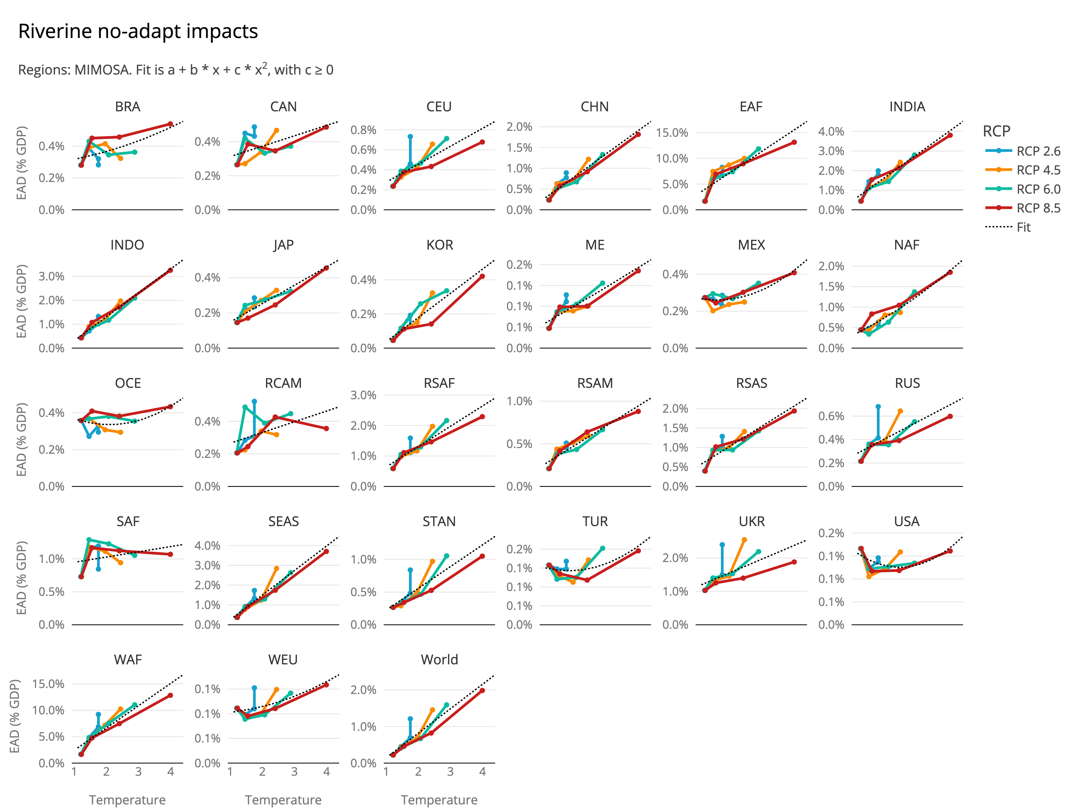
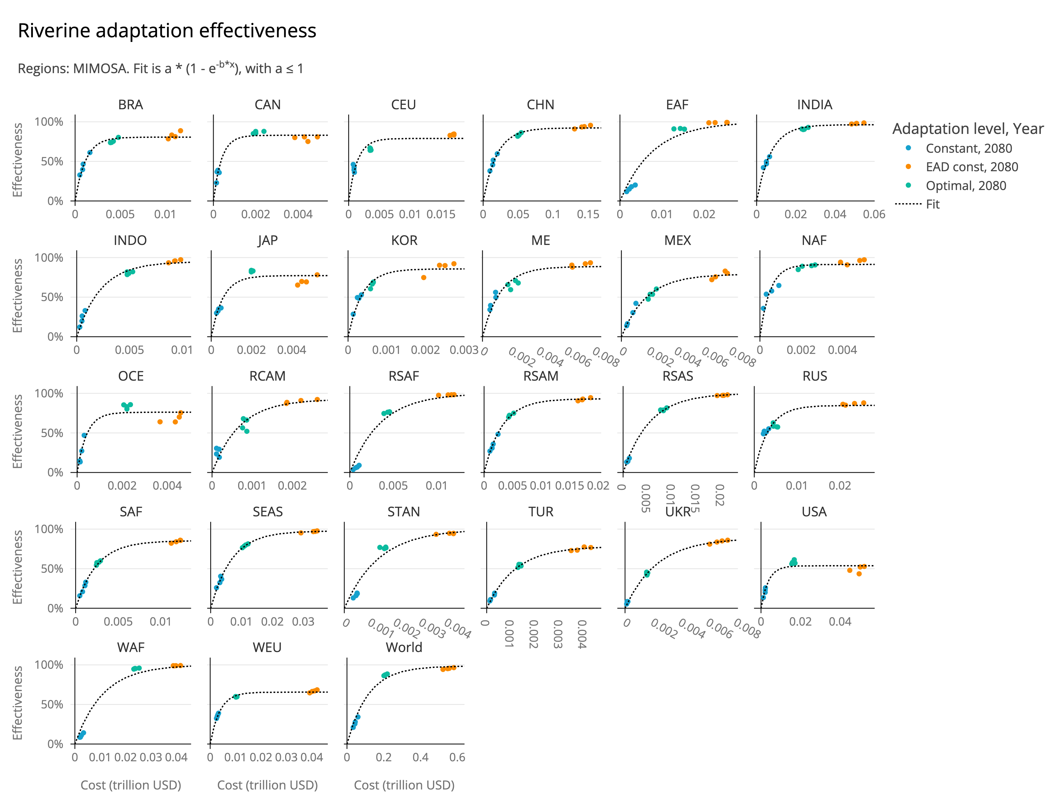
| Variables created in this module: |
|---|
riverine_damage_costs_gross: Gross damages from riverine flooding, without adaptation. |
riverine_adaptation_costs_abs: Absolute adaptation costs for riverine flooding, in currency units. Used to calculate the adaptation level. |
riverine_adaptation_costs: Adaptation costs for riverine flooding, as a fraction of GDP. |
riverine_adaptation_level: Adaptation level for riverine flooding, as a fraction of gross damages. 0 means that no damages are avoided, while 1 means that all damages are avoided. |
riverine_damage_costs: Residual damages from riverine flooding, after adaptation. If `noadaptation` is chosen, this variable represents the gross damages. |
Source code in mimosa/components/damages/accreu/riverine_flooding.py
30 31 32 33 34 35 36 37 38 39 40 41 42 43 44 45 46 47 48 49 50 51 52 53 54 55 56 57 58 59 60 61 62 63 64 65 66 67 68 69 70 71 72 73 74 75 76 77 78 79 80 81 82 83 84 85 86 87 88 89 90 91 92 93 94 95 96 97 98 99 100 101 102 103 104 105 106 107 108 109 110 111 112 113 114 115 116 117 118 119 120 121 122 123 124 125 126 127 128 129 130 131 132 133 134 135 136 137 138 139 140 141 142 143 144 145 146 147 148 149 150 151 152 153 154 155 156 157 158 159 160 161 162 163 164 165 166 167 168 169 170 171 172 173 174 175 176 177 178 179 180 181 182 183 184 185 186 187 188 189 190 191 192 193 194 195 196 197 198 199 200 201 202 203 204 205 206 207 208 209 210 211 212 213 214 215 216 217 218 219 220 221 222 223 224 225 226 227 228 229 230 231 232 233 234 235 236 | |
The impact of climate change on labour productivity can be decomposed in two types: heat-related expected annual costs due to warming (e.g. hot regions get hotter, leading to reduced labour productivity), and cold-related expected annual benefits due to less cold days (especially relevant for currently cold regions).
The heat-related gross damage costs are fitted using a linear function of global temperature, shifted to 0 at the start year.
The cold-related benefits of climate change are also fitted using a linear function of global temperature, and shifted to 0 at the start year.
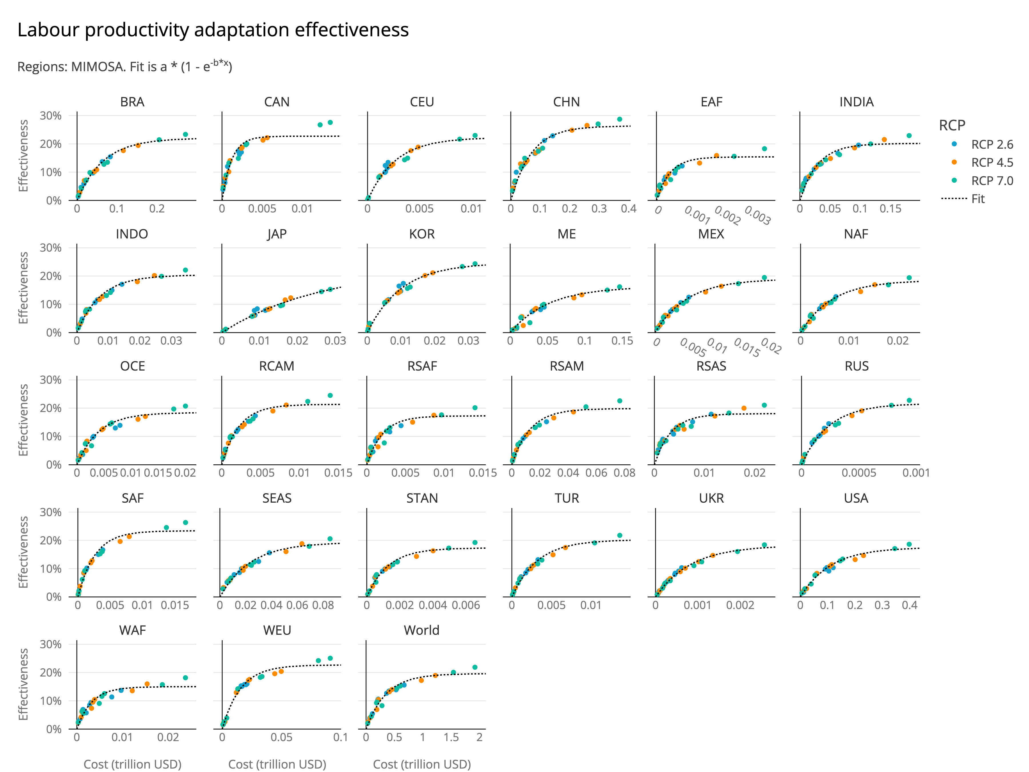
The adaptation function, which only applies to heat-related gross damages, is fitted with a negative-exponential saturation (NES) curve, like in all three sectors, using regional max. effectiveness and cost coefficient:
This leads to the residual, heat related damages:
The final, net damages are calculated as the sum of the heat-related residual damages and the cold-related benefits:
-
Global damages (heat- and cold-related, without adapt.)
-
Global adaptation costs (only for heat-related damages)
Regional damage and adaptation functions
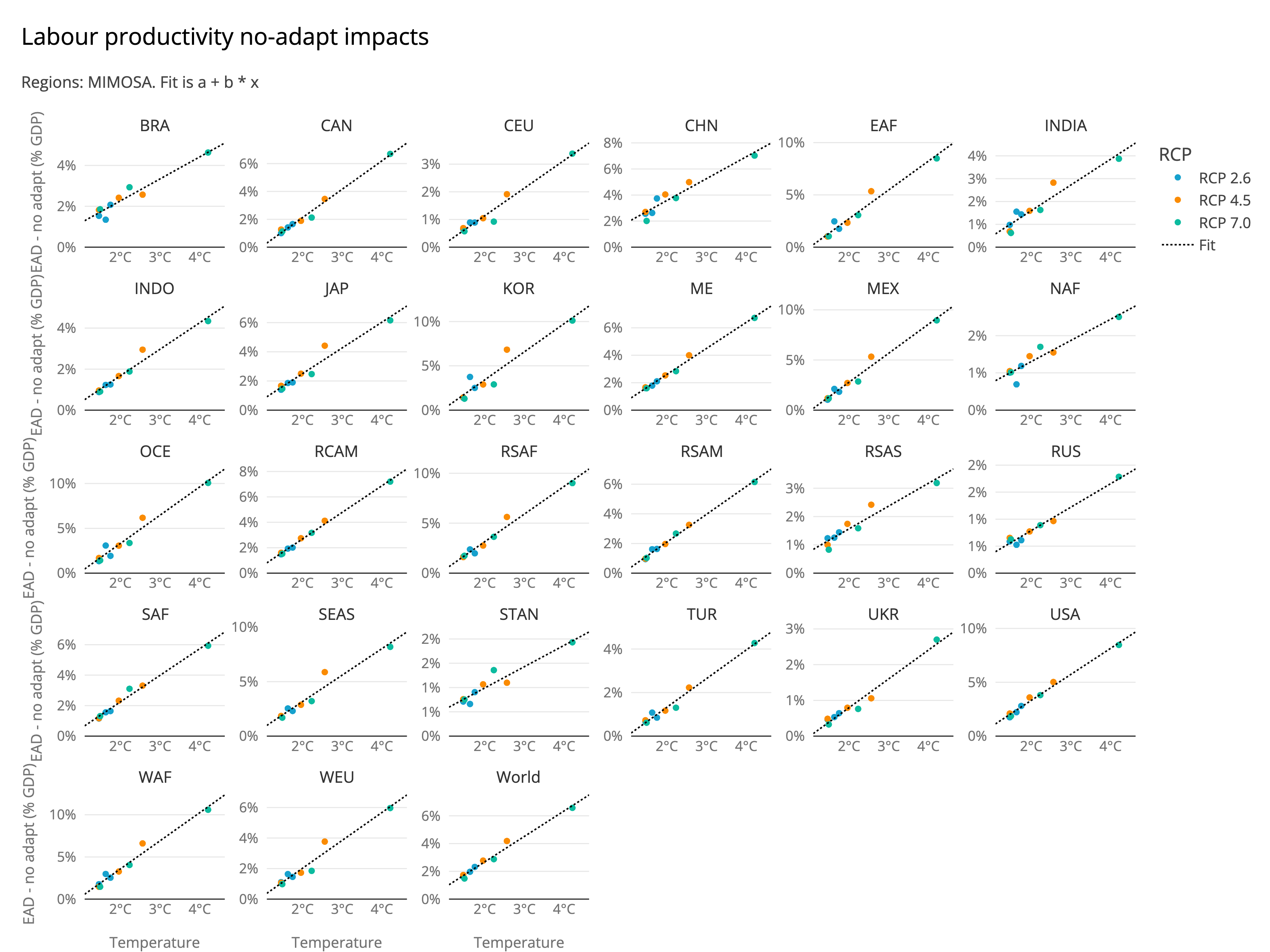
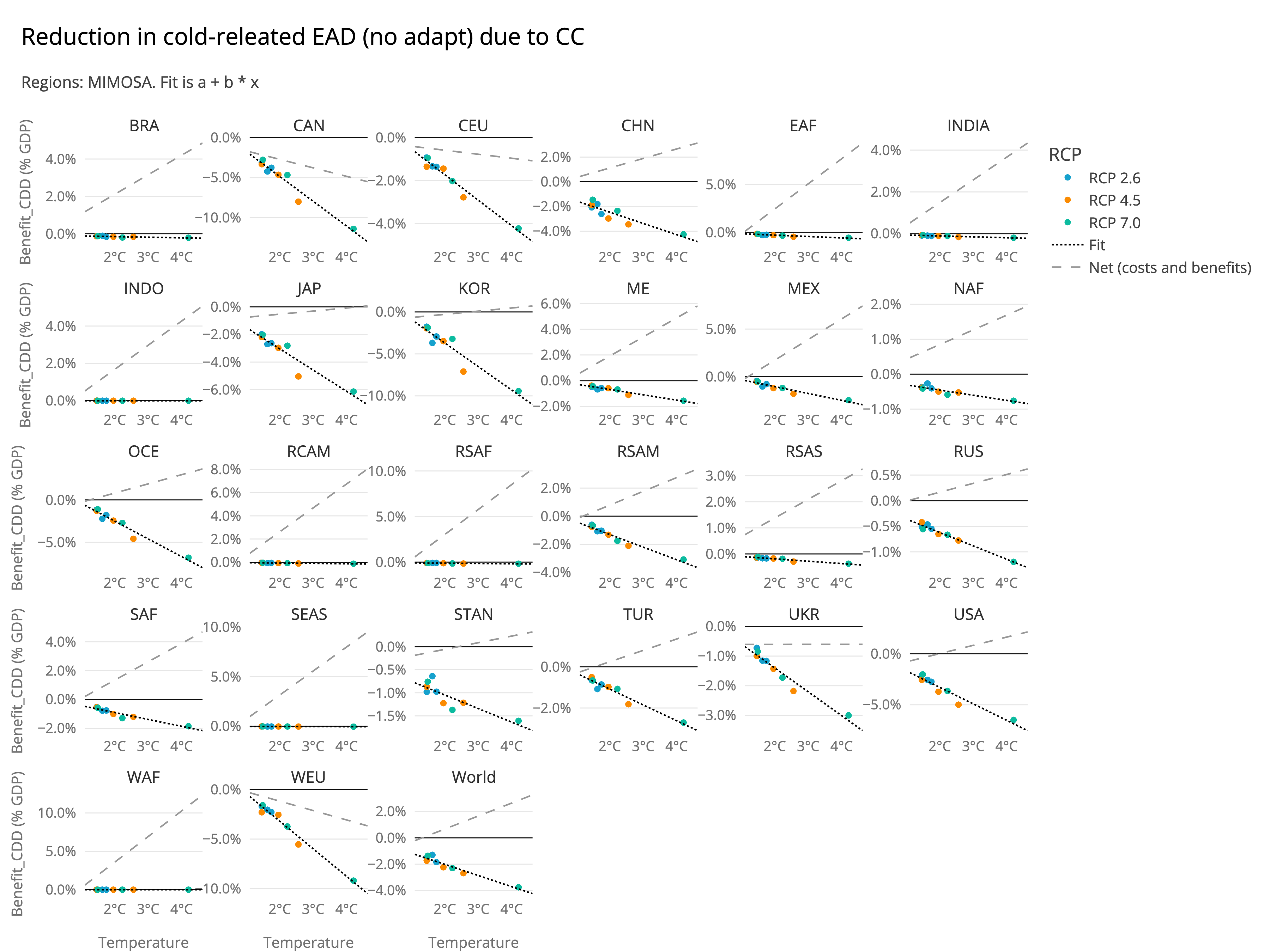
| Variables created in this module: |
|---|
labourprod_damage_costs_gross: Gross damages from heat-related labour productivity loss (e.g. hot regions get hotter), without adaptation |
labourprod_damage_costs_benefits: Benefits from reduced cold days for labour productivity (e.g. cold regions get less cold). No adaptation is applied to these benefits, as they are not related to heat stress. |
labourprod_adaptation_costs_abs: Adaptation costs for labour productivity (absolute values) (applied only to heat-related damages, not cold-related benefits) |
labourprod_adaptation_costs: Adaptation costs for labour productivity (as a fraction of GDP) (applied only to heat-related damages, not cold-related benefits) |
labourprod_adaptation_level: Adaptation level for labour productivity (applied only to heat-related damages, not cold-related benefits) |
labourprod_damage_costs: Residual damages for labour productivity after adaptation (heat-related component only) |
labourprod_damage_costs_net: Sum of heat-related residual damages and cold-related benefits for labour productivity (net damages) |
Source code in mimosa/components/damages/accreu/labour_productivity.py
31 32 33 34 35 36 37 38 39 40 41 42 43 44 45 46 47 48 49 50 51 52 53 54 55 56 57 58 59 60 61 62 63 64 65 66 67 68 69 70 71 72 73 74 75 76 77 78 79 80 81 82 83 84 85 86 87 88 89 90 91 92 93 94 95 96 97 98 99 100 101 102 103 104 105 106 107 108 109 110 111 112 113 114 115 116 117 118 119 120 121 122 123 124 125 126 127 128 129 130 131 132 133 134 135 136 137 138 139 140 141 142 143 144 145 146 147 148 149 150 151 152 153 154 155 156 157 158 159 160 161 162 163 164 165 166 167 168 169 170 171 172 173 174 175 176 177 178 179 180 181 182 183 184 185 186 187 188 189 190 191 192 193 194 195 196 197 198 199 200 201 202 203 204 205 206 207 208 209 210 211 212 213 214 215 216 217 218 219 220 221 222 223 224 225 226 227 228 229 230 231 232 233 234 235 236 237 238 239 240 241 242 243 244 245 246 247 248 249 250 251 252 253 254 255 256 257 258 259 260 261 262 263 264 265 266 267 268 269 270 271 272 273 274 275 276 277 278 279 280 281 282 283 284 285 286 287 288 289 290 291 292 293 294 295 296 297 | |
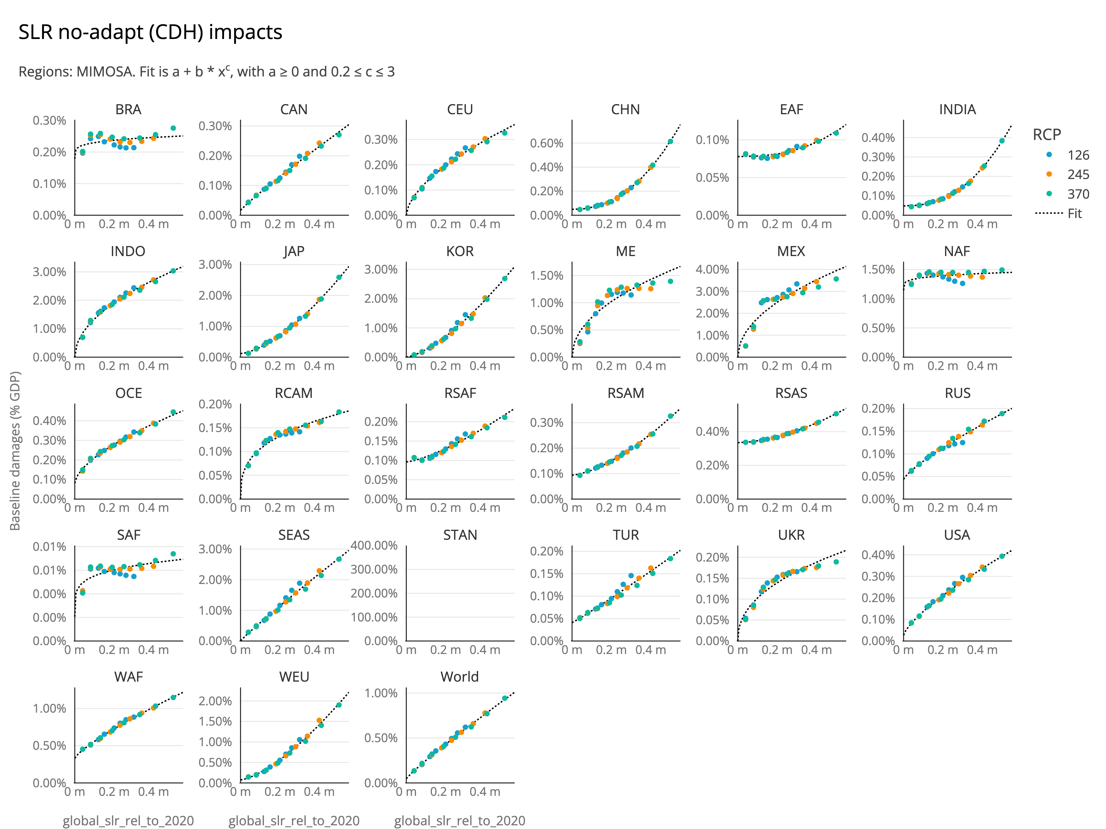
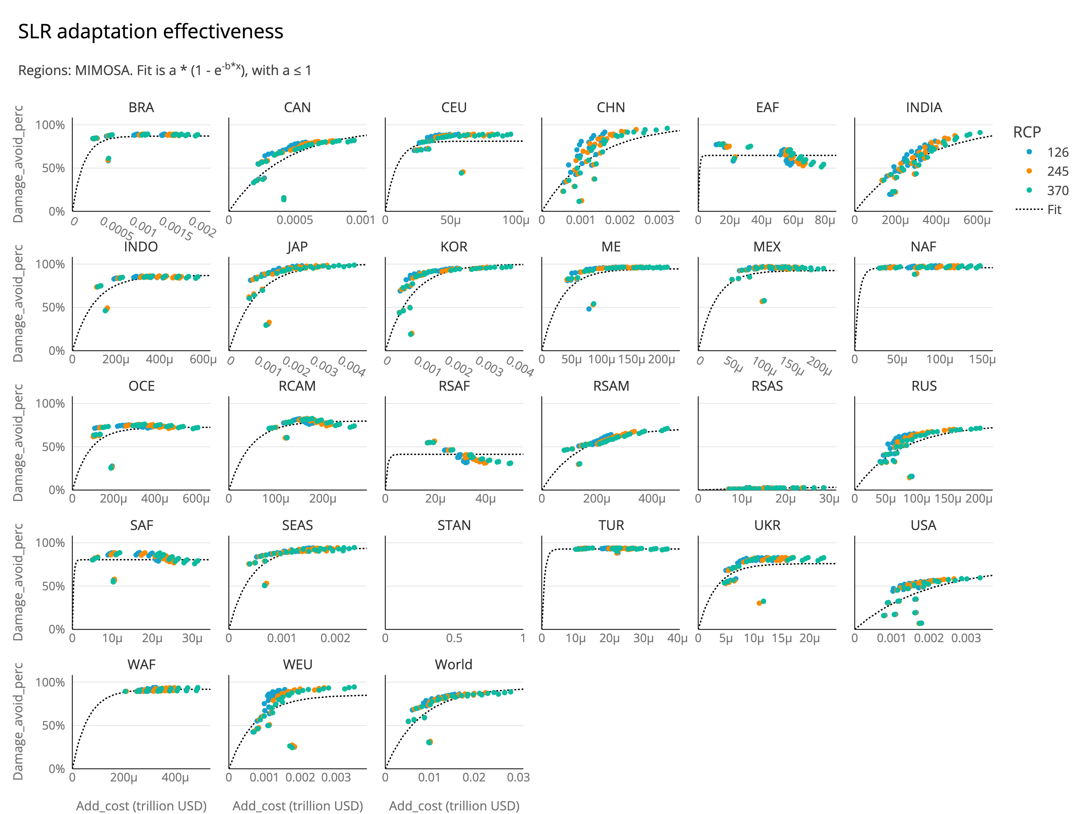
The sea-level rise impacts are calculated using the DIVA model. Specifically, for this purpose, we compare the Constant Dike Height scenario (“no adaptation / CDH”) with three adaptation scenarios: Constant flood protection standards, Doubling flood protection standards, and Quadrupling flood protection standards. Importantly, we do not use the “optimal adaptation” scenario from DIVA, to avoid double optimisation in the IAMs.
The gross damages are fitted with a power function of global sea-level rise:
The adaptation function is fitted with a negative-exponential saturation (NES) curve, like in all three sectors, using regional max. effectiveness and cost coefficient:
Subsequently, the residual damages are calculated as:
-
Global damages (without adaptation)
-
Global adaptation costs
Regional damage and adaptation functions
| Variables created in this module: |
|---|
slr_damage_costs_gross: Gross damages from sea-level rise, without adaptation |
slr_adaptation_costs_abs: Absolute adaptation costs for sea-level rise, in currency units. Used to calculate the adaptation level |
slr_adaptation_costs: Adaptation costs for sea-level rise, as a fraction of GDP. |
slr_adaptation_level: Adaptation level for sea-level rise, as a fraction of gross damages. 0 means that no damages are avoided, while 1 means that all damages are avoided. |
slr_damage_costs: Residual damages from sea-level rise, after adaptation. If `noadaptation` is chosen, this variable represents the gross damages. |
Source code in mimosa/components/damages/accreu/sealevelrise.py
31 32 33 34 35 36 37 38 39 40 41 42 43 44 45 46 47 48 49 50 51 52 53 54 55 56 57 58 59 60 61 62 63 64 65 66 67 68 69 70 71 72 73 74 75 76 77 78 79 80 81 82 83 84 85 86 87 88 89 90 91 92 93 94 95 96 97 98 99 100 101 102 103 104 105 106 107 108 109 110 111 112 113 114 115 116 117 118 119 120 121 122 123 124 125 126 127 128 129 130 131 132 133 134 135 136 137 138 139 140 141 142 143 144 145 146 147 148 149 150 151 152 153 154 155 156 157 158 159 160 161 162 163 164 165 166 167 168 169 170 171 172 173 174 175 176 177 178 179 180 181 182 183 184 185 186 187 188 189 190 191 192 193 194 195 196 197 198 199 200 201 202 203 204 205 206 207 208 209 210 211 212 213 214 215 216 217 218 219 220 221 222 223 224 225 226 227 228 229 230 231 232 233 234 235 | |
Physical impacts
The ACCREU damage representation includes temperature-related mortality impacts, though without accounting for explicit adaptation. Like labour productivity, there is a heat-related and cold-related component, varying strongly between regions. As global mean temperature increases, the heat-related mortality increases, while the cold-related mortality decreases.
The mortality forecasts are sourced from Bressler et al. (2021). The paper forecasts the change in future heat-related and cold-related mortality rates under RCP 2.6, RCP 4.5, RCP 6.0 and RCP 8.5 scenarios. It does so for the 2040-59 and 2080-99 periods. For this analysis, the estimates for these ranges are assigned to the years 2050 and 2090 respectively. In order to convert the forecasted change in the mortality rate into an estimate of excess mortality, the Bressler forecasts were combined with mortality rate forecasts from the World Bank (2025).
The heat-related mortality (as % of population) was fitted with a quadratic function. Given that they represent additional mortality relative to 2010, the fit was relative to temperature in 2010: 1.1 °C. To obtain a mortality value in absolute numbers, we multiply by total population:
Cold-related mortality showed a linear relation with temperature, accounting for the fact that reductions in cold-related mortality don't become marginally larger when temperatures become very high. In fact, at some point we expect to see a plateau. However, the data doesn't show this behaviour for the assessed temperature range, where a linear fit throughout is the best fit:
The total mortality is the sum of both:
-
Global mortality (heat- and cold-related, without adaptation)
| Variables created in this module: |
|---|
mortality_heat_related: Extra heat-related mortality, in absolute numbers. Extra is compared to start year of the run (2025). |
mortality_cold_related: Reduced cold-related mortality, in absolute numbers, compared to start year of the run (2025). |
mortality_net: Sum of extra heat-related mortality and reduced cold-related mortality, in absolute numbers. |
Monetisation of mortality
If the MIMOSA parameter monetise mortality is set to true, the mortality values are converted to monetary value, which are then used by the welfare function:
params = load_params()
params["economics"]["damages"]["accreu"]["monetise_mortality"] = True # or False
model = MIMOSA(params)
Valuation of mortality in monetary units can be done using values of statistical life (VSL) or values of statistical life years (VSLY) multiplied by the expected life years lost. The main difference between these valuation methods is that the VSLY approach gives relatively lower values to mortality of people with a lower remaining life expectancy, while the VSL approach values mortality in all age classes equally.
Here, we follow the recommendation by the OECD to not adjust valuation according to the age of the population as this would imply that public policy and cost-benefit analysis outcomes could differ solely based on differences in the age of the populations studied. Moreover, little is known about the expected life years lost due to climate change impacts (Toulemon & Barbieri, 2008).
We therefore use the VSL approach for valuing the cost of mortality. The default MIMOSA value is the recommended estimates of the VSL from the OECD (2025). They provide a weighted world value of the VSL of 2.4 million dollars, which gives a \(\text{VSL}_{\text{rel}}\) of 117.59 times the GDP per capita.
The VSL in dollar terms is therefore:
The resulting mortality costs (in absolute terms) are given by:
Since these are the only non-market damages in the model, the non-market damages are equal to the mortality costs. These are not subtracted from GDP, but are removed in the welfare function. damages.
| Variables created when mortality is monetised: |
|---|
mortality_vsl: Value of statistical life (VSL) in currency units, calculated as the relative VSL times GDP per capita |
mortality_damage_costs_abs: Mortality damage costs in currency units. Since the extra heat-related deaths and reduced cold-related deaths are considered, this value can be positive or negative, depending on the region, time, and temperature. |
mortality_damage_costs: Mortality damage costs expressed as % of GDP |
Source code in mimosa/components/damages/accreu/mortality.py
199 200 201 202 203 204 205 206 207 208 209 210 211 212 213 214 215 216 217 218 219 220 221 222 223 224 225 226 227 228 229 230 231 232 233 234 235 236 237 238 239 240 241 242 243 244 245 246 247 248 249 250 251 252 253 254 255 256 257 258 259 260 261 262 263 264 265 266 267 268 269 270 271 272 273 274 275 276 277 278 279 280 281 282 283 284 285 286 287 288 289 290 291 292 293 294 295 296 297 298 299 300 301 302 303 304 305 306 307 308 309 310 | |
Source code in mimosa/components/damages/accreu/mortality.py
25 26 27 28 29 30 31 32 33 34 35 36 37 38 39 40 41 42 43 44 45 46 47 48 49 50 51 52 53 54 55 56 57 58 59 60 61 62 63 64 65 66 67 68 69 70 71 72 73 74 75 76 77 78 79 80 81 82 83 84 85 86 87 88 89 90 91 92 93 94 95 96 97 98 99 100 101 102 103 104 105 106 107 108 109 110 111 112 113 114 115 116 117 118 119 120 121 122 123 124 125 126 127 128 129 130 131 132 133 134 135 136 137 138 139 140 141 142 143 144 145 146 147 148 149 150 151 152 153 154 155 156 157 158 159 160 161 162 163 164 165 166 167 168 169 170 171 172 173 174 175 176 177 178 179 180 181 182 183 184 185 186 187 188 189 190 191 192 193 194 195 196 | |
Total damages and adaptation
The total damage costs are the sum of the sectoral damages:
Similarly, if adaptation is enabled, the total adaptation costs are the sum of the sectoral adaptation costs:
As mentioned above, mortality is also included in this damage representation. However, since (the monetisation of) mortality
is not represented as a direct cost to the economy, but rather a non-market impact, it is not included in the total damage costs.
Instead, the monetised mortality costs are reported separately. If a user is interested in the sum of market and non-market damages,
this is given by the variable market_and_non_market_damage_costs, calculated as:
where \(\text{abs. damages}_{\text{mortality}}\) is the mortality damages in absolute terms (i.e. in currency units), and \(\text{GDP}_{\text{gross}}\) is the gross GDP, also in absolute terms (i.e. in currency units).
| Variables created in this module: |
|---|
damage_costs: Total damages from all sectors (excluding non-market impacts like mortality), as a fraction of GDP. |
damage_costs_abs: Total damages from all sectors (excluding non-market impacts like mortality), in currency units. |
global_damage_costs: Global total damages from all sectors (excluding non-market impacts like mortality), as a fraction of global GDP. |
adaptation_costs: Total adaptation costs from all sectors, as a fraction of GDP. |
adaptation_costs_abs: Total adaptation costs from all sectors, in currency units. |
global_adaptation_costs: Global total adaptation costs from all sectors, as a fraction of global GDP. |
non_market_damage_costs_abs: Total non-market damages (monetised mortality), in currency units. |
market_and_non_market_damage_costs_abs: Total market and non-market damages, in currency units. |
market_and_non_market_damage_costs: Total market and non-market damages, as a fraction of GDP. |
Source code in mimosa/components/damages/accreu/all_damages.py
34 35 36 37 38 39 40 41 42 43 44 45 46 47 48 49 50 51 52 53 54 55 56 57 58 59 60 61 62 63 64 65 66 67 68 69 70 71 72 73 74 75 76 77 78 79 80 81 82 83 84 85 86 87 88 89 90 91 92 93 94 95 96 97 98 99 100 101 102 103 104 105 106 107 108 109 110 111 112 113 114 115 116 117 118 119 120 121 122 123 124 125 126 127 128 129 130 131 132 133 134 135 136 137 138 139 140 141 142 143 144 145 146 147 148 149 150 151 152 153 154 155 156 157 158 159 160 161 162 163 164 165 166 167 168 169 170 171 172 173 174 175 176 177 178 179 180 181 182 183 184 185 186 187 188 189 190 191 192 193 194 195 196 197 198 199 200 201 202 203 204 205 206 207 208 209 210 211 212 213 214 215 216 217 218 219 220 221 222 223 224 225 226 227 228 229 230 231 232 233 234 235 236 237 238 239 240 241 242 243 244 245 246 247 248 249 250 251 252 253 254 255 256 257 258 259 260 261 262 263 264 265 266 267 268 269 270 271 272 273 274 275 276 277 278 279 280 281 | |