8 Combining DataFrames

Previously, we have seen how to analyze and manipulate data in a single DataFrame. However, you will often find data saved into different files and, therefore, you may need to deal with several different pandas DataFrames.
In this session we will explore different ways of combining DataFrames into a single DataFrame.

Let’s start loading the pandas library, reading two data sets into DataFrames, and having a quick look at the tabular data: surveys.csv and species.csv

import pandas as pd

surveys_df = pd.read_csv("../course_materials/data/surveys.csv", keep_default_na=False, na_values=[""])
species_df = pd.read_csv("../course_materials/data/species.csv", keep_default_na=False, na_values=[""])

print(surveys_df.info())
surveys_df.head()

<class 'pandas.core.frame.DataFrame'>
RangeIndex: 35549 entries, 0 to 35548
Data columns (total 9 columns):
 #   Column           Non-Null Count  Dtype  
---  ------           --------------  -----  
 0   record_id        35549 non-null  int64  
 1   month            35549 non-null  int64  
 2   day              35549 non-null  int64  
 3   year             35549 non-null  int64  
 4   plot_id          35549 non-null  int64  
 5   species_id       34786 non-null  object 
 6   sex              33038 non-null  object 
 7   hindfoot_length  31438 non-null  float64
 8   weight           32283 non-null  float64
dtypes: float64(2), int64(5), object(2)
memory usage: 2.4+ MB
None

	record_id	month	day	year	plot_id	species_id	sex	hindfoot_length	weight
0	1	7	16	1977	2	NL	M	32.0	NaN
1	2	7	16	1977	3	NL	M	33.0	NaN
2	3	7	16	1977	2	DM	F	37.0	NaN
3	4	7	16	1977	7	DM	M	36.0	NaN
4	5	7	16	1977	3	DM	M	35.0	NaN

print(species_df.info())
species_df.head()

<class 'pandas.core.frame.DataFrame'>
RangeIndex: 54 entries, 0 to 53
Data columns (total 4 columns):
 #   Column      Non-Null Count  Dtype 
---  ------      --------------  ----- 
 0   species_id  54 non-null     object
 1   genus       54 non-null     object
 2   species     54 non-null     object
 3   taxa        54 non-null     object
dtypes: object(4)
memory usage: 1.8+ KB
None

	species_id	genus	species	taxa
0	AB	Amphispiza	bilineata	Bird
1	AH	Ammospermophilus	harrisi	Rodent
2	AS	Ammodramus	savannarum	Bird
3	BA	Baiomys	taylori	Rodent
4	CB	Campylorhynchus	brunneicapillus	Bird

We now have two DataFrames. The first, surveys_df, contains information on individuals of a species recorded in a survey, while the second, species_df, contains more detailed information on each species.

8.1 Concatenating DataFrames

The first way we will combine DataFrames is concatenation, i.e. simply putting DataFrames one after the other either vertically or horizontally.

Concatenation can be used if the DataFrames are similar, meaning that they either have the same rows or columns. We will see examples of this later.

To concatenate two DataFrames you will use the function pd.concat(), specifying as arguments the DataFrames to concatenate and axis=0 or axis=1 for vertical or horizontal concatenation, respectively.

We will only be looking at vertical concatenation, but it is good to be aware that there is more to be discovered beyond what we describe here.

Let us first obtain two small DataFrames from the larger surveys_df dataset.

# Subsetting DataFrames
surveys_df_sub_first10 = surveys_df.head(10)
surveys_df_sub_last10  = surveys_df.tail(10)

We now have two DataFrames, one with the first ten rows of the original dataset, and another with the last ten rows.

Now, let us do some vertical concatenation or stacking. In this case the two DataFrames are simply stacked ‘on top of’ each other (remember to specify axis=0).

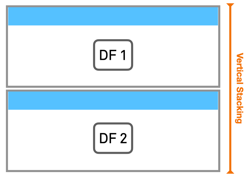
Vertical stacking can be understood as combining two DataFrames that have different sets of the same type of data. In our example, it may be that one field researcher has registered the first ten entries, and another did the last ten, both using the same laboratory sheets. They both wrote down the same information (weight, species, and so on) of all different individuals. If we combine them, we have one list of twenty records, rather than two lists of ten.

# Stack the DataFrames on top of each other
vertical_stack = pd.concat([surveys_df_sub_first10, surveys_df_sub_last10], axis=0)

print(vertical_stack.info())
vertical_stack

<class 'pandas.core.frame.DataFrame'>
Int64Index: 20 entries, 0 to 35548
Data columns (total 9 columns):
 #   Column           Non-Null Count  Dtype  
---  ------           --------------  -----  
 0   record_id        20 non-null     int64  
 1   month            20 non-null     int64  
 2   day              20 non-null     int64  
 3   year             20 non-null     int64  
 4   plot_id          20 non-null     int64  
 5   species_id       19 non-null     object 
 6   sex              16 non-null     object 
 7   hindfoot_length  15 non-null     float64
 8   weight           6 non-null      float64
dtypes: float64(2), int64(5), object(2)
memory usage: 1.6+ KB
None

	record_id	month	day	year	plot_id	species_id	sex	hindfoot_length	weight
0	1	7	16	1977	2	NL	M	32.0	NaN
1	2	7	16	1977	3	NL	M	33.0	NaN
2	3	7	16	1977	2	DM	F	37.0	NaN
3	4	7	16	1977	7	DM	M	36.0	NaN
4	5	7	16	1977	3	DM	M	35.0	NaN
5	6	7	16	1977	1	PF	M	14.0	NaN
6	7	7	16	1977	2	PE	F	NaN	NaN
7	8	7	16	1977	1	DM	M	37.0	NaN
8	9	7	16	1977	1	DM	F	34.0	NaN
9	10	7	16	1977	6	PF	F	20.0	NaN
35539	35540	12	31	2002	15	PB	F	26.0	23.0
35540	35541	12	31	2002	15	PB	F	24.0	31.0
35541	35542	12	31	2002	15	PB	F	26.0	29.0
35542	35543	12	31	2002	15	PB	F	27.0	34.0
35543	35544	12	31	2002	15	US	NaN	NaN	NaN
35544	35545	12	31	2002	15	AH	NaN	NaN	NaN
35545	35546	12	31	2002	15	AH	NaN	NaN	NaN
35546	35547	12	31	2002	10	RM	F	15.0	14.0
35547	35548	12	31	2002	7	DO	M	36.0	51.0
35548	35549	12	31	2002	5	NaN	NaN	NaN	NaN

The resulting DataFrame (vertical_stack) consists, as expected, of 20 rows. These are the result of the first and last 10 rows of our original DataFrame surveys_df.

You may have noticed that the last ten rows have very high index, not consecutive with the first ten rows. This is because concatenation preserves the indices of the two original DataFrames. If you want a brand new set of indices for your concateneted DataFrame, simply reset the indices using the method .reset_index(). Notice that this adds a column index to your DataFrame, that maintains the original index. If you pass drop=True into the function, you will avoid the addition of this column.

vertical_stack.reset_index()

	index	record_id	month	day	year	plot_id	species_id	sex	hindfoot_length	weight
0	0	1	7	16	1977	2	NL	M	32.0	NaN
1	1	2	7	16	1977	3	NL	M	33.0	NaN
2	2	3	7	16	1977	2	DM	F	37.0	NaN
3	3	4	7	16	1977	7	DM	M	36.0	NaN
4	4	5	7	16	1977	3	DM	M	35.0	NaN
5	5	6	7	16	1977	1	PF	M	14.0	NaN
6	6	7	7	16	1977	2	PE	F	NaN	NaN
7	7	8	7	16	1977	1	DM	M	37.0	NaN
8	8	9	7	16	1977	1	DM	F	34.0	NaN
9	9	10	7	16	1977	6	PF	F	20.0	NaN
10	35539	35540	12	31	2002	15	PB	F	26.0	23.0
11	35540	35541	12	31	2002	15	PB	F	24.0	31.0
12	35541	35542	12	31	2002	15	PB	F	26.0	29.0
13	35542	35543	12	31	2002	15	PB	F	27.0	34.0
14	35543	35544	12	31	2002	15	US	NaN	NaN	NaN
15	35544	35545	12	31	2002	15	AH	NaN	NaN	NaN
16	35545	35546	12	31	2002	15	AH	NaN	NaN	NaN
17	35546	35547	12	31	2002	10	RM	F	15.0	14.0
18	35547	35548	12	31	2002	7	DO	M	36.0	51.0
19	35548	35549	12	31	2002	5	NaN	NaN	NaN	NaN

8.2 Joining DataFrames

Concatenating DataFrames allows you to combine two entire DataFrames into a single one. In many cases, you want to combine only selected parts of two DataFrames.

You might, for example, want to merge rows of two DataFrames that have matching values in specific columns. The pandas function merge() performs an operation that you may know as a join if you worked with databases before. The join operation joins the content of two DataFrames in a particular way. There are different types of joins, but the workflow to perform a join operation is always the same:

You identify a left and a right DataFrame, among the two you want to join;
You identify in both your left and right DataFrame a column (or set of columns) to join on;
You choose the type of join;
You perform the join running the function pd.merge() with the specified inputs and options.

What it means for a DataFrame to be ‘left’ or ‘right’ depends on the type of join. The main thing to remember is that it matters which DataFrame you mention first when performing a join.

We will only be looking at what is know as an inner join. Investigating the other types of joins is left as an exercise.

Let’s see some join example using the first ten rows of our surveys_df DataFrame (surveys_df_sub_first10). This will be our left DataFrame, containing data on individual animals. Our right DataFrame will be the first 20 rows of species_df, containing some information on each species. Let us rename them for the purpose of the join:

left_df = surveys_df_sub_first10
right_df = species_df.head(20)

left_df

	record_id	month	day	year	plot_id	species_id	sex	hindfoot_length	weight
0	1	7	16	1977	2	NL	M	32.0	NaN
1	2	7	16	1977	3	NL	M	33.0	NaN
2	3	7	16	1977	2	DM	F	37.0	NaN
3	4	7	16	1977	7	DM	M	36.0	NaN
4	5	7	16	1977	3	DM	M	35.0	NaN
5	6	7	16	1977	1	PF	M	14.0	NaN
6	7	7	16	1977	2	PE	F	NaN	NaN
7	8	7	16	1977	1	DM	M	37.0	NaN
8	9	7	16	1977	1	DM	F	34.0	NaN
9	10	7	16	1977	6	PF	F	20.0	NaN

right_df

	species_id	genus	species	taxa
0	AB	Amphispiza	bilineata	Bird
1	AH	Ammospermophilus	harrisi	Rodent
2	AS	Ammodramus	savannarum	Bird
3	BA	Baiomys	taylori	Rodent
4	CB	Campylorhynchus	brunneicapillus	Bird
5	CM	Calamospiza	melanocorys	Bird
6	CQ	Callipepla	squamata	Bird
7	CS	Crotalus	scutalatus	Reptile
8	CT	Cnemidophorus	tigris	Reptile
9	CU	Cnemidophorus	uniparens	Reptile
10	CV	Crotalus	viridis	Reptile
11	DM	Dipodomys	merriami	Rodent
12	DO	Dipodomys	ordii	Rodent
13	DS	Dipodomys	spectabilis	Rodent
14	DX	Dipodomys	sp.	Rodent
15	EO	Eumeces	obsoletus	Reptile
16	GS	Gambelia	silus	Reptile
17	NL	Neotoma	albigula	Rodent
18	NX	Neotoma	sp.	Rodent
19	OL	Onychomys	leucogaster	Rodent

The column we want to perform the join on is the one containing information about the species_id. Conveniently, this column has the same label in both DataFrames. Note that this is not always the case.

inner_join = pd.merge(left_df, right_df, left_on='species_id', right_on='species_id', how='inner')
inner_join

	record_id	month	day	year	plot_id	species_id	sex	hindfoot_length	weight	genus	species	taxa
0	1	7	16	1977	2	NL	M	32.0	NaN	Neotoma	albigula	Rodent
1	2	7	16	1977	3	NL	M	33.0	NaN	Neotoma	albigula	Rodent
2	3	7	16	1977	2	DM	F	37.0	NaN	Dipodomys	merriami	Rodent
3	4	7	16	1977	7	DM	M	36.0	NaN	Dipodomys	merriami	Rodent
4	5	7	16	1977	3	DM	M	35.0	NaN	Dipodomys	merriami	Rodent
5	8	7	16	1977	1	DM	M	37.0	NaN	Dipodomys	merriami	Rodent
6	9	7	16	1977	1	DM	F	34.0	NaN	Dipodomys	merriami	Rodent

As you may notice, the resulting DataFrame has only seven rows, while our original DataFrames had 10 and 20 rows, respectively. This is because an inner join selects only those rows where the value of the joined column occurs in both DataFrames (mathematically, an intersection).

Aside from the inner join, there are three more types of join that you can do using the merge() function: - An inner join selects only the rows that result from the combination of matching rows in both the original left and right DataFrames (intersection); - A left join selects all rows that were in the original left DataFrame, some of which may have been joined with a matching entry from the right DataFrame; - A right join selects all rows that were in the original right DataFrame, some of which may have been joined with a matching entry from the left DataFrame; - An outer join merges the two DataFrames and keeps all resulting rows.

To better understand how join works, it may be useful to look at the diagrams below:

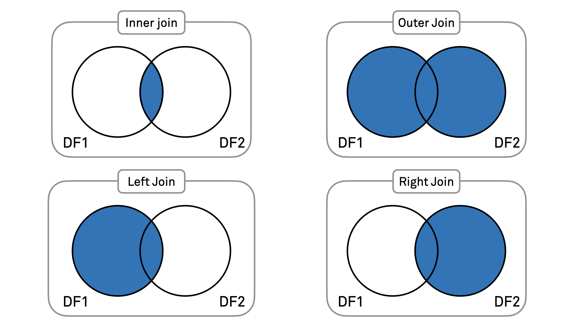
Do you want to select only common information between the two DataFrames? Then you use an inner join;
Do you want to add information to your left DataFrame? Then you use a left join;
Do you want to add information to your right DataFrame? Then you use a right join;
Do you want to get all the information from the two DataFrames? Then you use an outer join.

Exercises 9 and 10

Now go to the Jupyter Dashboard in your internet browser and continue with exercise 9 and 10.

We will continue with Data visualization.