import pandas as pd
import matplotlib.pyplot as plt
import numpy as np
import scipy.stats as statsStarting to work with Pandas
Background to this example
When working in Python for data analysis, the Pandas packages is one most commonly used packages. Pandas is a fast, powerful, flexible and easy to use open source data analysis and manipulation tool, built on top of the Python programming language. It allows you to load, manipulate, analyse, visualize and write data in other file formats and ways than the original data.
In this practical you will learn about
Explore data
Manipulating data
Dealing with missing values
Simple visuals
Working with categorical data
Getting started
In this practical we will start exploring some of the basic functions in Pandas, learn about the different formats and ways you can use Pandas.
There are lots of resources to help you with using Pandas and provide nice tips, trick and examples. For example you can use a cheat sheet to quickly remember and double check which functions to use (e.g. https://pandas.pydata.org/Pandas_Cheat_Sheet.pdf) or useful pages that describe the most basic functions of Pandas. You can also find lots of good examples that use Pandas online for different types of data and types of analyses (https://realpython.com/search?q=pandas).
Let’s start with using Python again by opening your Conda environment and then opening Spyder (for detailed instructions please look back at the instruction guide). We start by loading some of the standard libraries in this course. We use:
Pandas (data management and data handling)
Numpy (statistical analysis and data handling)
Matplotlib (plotting)
Scipy (statistical analysis)
Importing packages
After you put these lines in your script potentially a small warning message might pop up, “… is imported but unused” this message is normal and just a message that the package isn’t used yet in your scripts.
Set the Working Directory
In Python you have to let the script know where to find the data that you want to use. This can be done using two ways, either by specifying relative filepaths or absolute filepaths.
In Spyder, the working directory is shown at the top right of the window under files. In this place you can navigate to your working directory. All relative paths are based on this directory.
You can also set it programmatically:
import os
os.chdir("your/desired/path")
print(os.getcwd())
An absolute path points to a file from the root of the filesystem and works regardless of the script’s location.
# macOS / Linux
file_path = "/Users/yourname/Documents/data/file.csv"

# Windows
file_path = "C:\\Users\\yourname\\Documents\\data\\file.csv"
The advantage of relative file paths is that if you move the folder in which you are working, all relative path stay the same and don’t need changing. The advantage of an absolute path is that it is easier to navigate if the data is in a completely different location or far outside of the working directory.
In general you should aim to use relative paths as the chance of making mistakes is reduced when moving data between computers or on your system.
In the working directory for example “UU/Data2/” you create a folder”Data”, this folder can contain all the .csv and other input files. For detailed instructions on downloading all necessary input data, please refer to the installation instructions.
Also create another folder with all called Scripts this folder can contain all the practicals. You can name them “Week01.py”,”Week02.py” etc. This way you can always run them an understand as well as find them back.
Running the Python code and making your script file
When you do the practical we want you to make a script file that contains all the code that you have created. To this end we will make use of a script file which is typically called something like Week01.py or Week02.py etc. These script files should contain all necessary code to reproduce your figures and findings. For example:
import pandas as pd
import matplotlib.pyplot as plt
import numpy as np
import scipy.stats as stats
import os

## Change to working dir
os.chdir("your/desired/path")

## Question 1
np.random.seed(1)
randomData_1 = np.random.normal(loc=0, scale=1, size=100)
randomData_2 = np.random.normal(loc=0, scale=1, size=100)
## Answer 1
## I think this is because x, y, z
....
....
....
You can use ## to put comments in the script or answers to the questions as is done in the example above.
If you want to run (parts of) your code you can use two options in Spyder. Either you run the entire script, however this will not print any output by default or you can run parts of your script and generate the outputs. To do this you can use these buttons in the program that can be found on the top left of the menu bar.

If you run the entire code it is recommended that you use print statements in your code as provided in the template below.
import pandas as pd
import matplotlib.pyplot as plt
import numpy as np
import scipy.stats as stats
import os

## Change to working dir
os.chdir("your/desired/path")

## Question 1
np.random.seed(1)
randomData_1 = np.random.normal(loc=0, scale=1, size=100)
randomData_2 = np.random.normal(loc=0, scale=1, size=100)
print(randomData_1)
print(randomData_2)
## Answer 1
## I think this is because x, y, z
....
....
....
This will ensure that randomData_1 and randomData_2 are printed even if you run the entire script. For efficiency reason we always recommended only the selection of code that you need to run rather than the entire script. It is expected that you hand in the .py files at the end of each week and that these files can run without errors.
Making your first dataframe
Let us first generate some random numbers to work with, for that we sample from normal distribution with mean (\(\mu\)) = 0 and a standard deviation (\(\sigma\)) of 1. For this we use the Numpy package and more specifically the function random.normal. We will create two random datasets to play around with and explore the potential of Pandas. For the purpose of this tutorial we also set the seed of the random number generator. A random seed (or seed state, or just seed) is a number (or vector) used to initialize a pseudorandom number generator. This ensure that when we select the random numbers in for example a exercise like this we always draw the same “random” numbers, and results are comparable between students.
np.random.seed(1)
randomData_1 = np.random.normal(loc=0, scale=1, size=100)
randomData_2 = np.random.normal(loc=0, scale=1, size=100)
Then we put the the random data into a Pandas Dataframe for easier manipulation. For this we merge the two datasets together, labeling the first one as ‘A’ and the second dataset as ‘B’.
df = pd.DataFrame({'A':randomData_1, 'B':randomData_2}, columns=['A','B'])When you look at the Dataframe you will see a couple of typical Pandas things, firstly you see the randomly generated numbers, you see the column labels ‘A’ and ‘B’ and lastly you see the numbers 0 to 99 indicating the rows numbers or in this case also the index of the dataframe. Both the index and the columns are very important elements as they provide unique identifiers for each individual data entry in the dataframe, a bit like coordinates on a map. Also note that Python (and thus Pandas) by defaults start counting at 0 rather than 1 which is sometimes the case for other programming languages.
The index and column names can be changed with the rename and set_index function. Use the function pages you can try and follow the examples below
df = df.rename(columns={"B":"C"})Or changing the index using
df = df.set_index(np.arange(10,110))You will see now that the index have changed, ranging from 10 to 109 rather than 0 to 99 before. One of the powerful characteristics of Pandas is that it can also use dates as an index and that you can use these to do some time operations. To make a string of correctly formatted dates, you can use the date_range function. The function requires either a start and end date or a length and frequency of the date format. If you look at the example below you see that we use the len function to find the total number of rows and we use the freq = ‘D’ which gives daily values. You can try changing it to other frequencies as well, like for example ‘W’ for weekly or ‘Y’ for yearly (more options can be found here). We give an example below
df = df.set_index(pd.date_range(start='1/1/2020', periods=len(df), freq='D'))Now we can do all kind of things to explore or manipulate the data. Firstly we can look at some common statistical properties, like the mean, min, max or median values of rows and columns.
df.mean()A 0.060583
C 0.152795
dtype: float64This will give you the mean over the columns. As you can see in the documentation of Pandas mean you can also specify the axis which is set by default to 0, which means that it will take the mean over the different rows/indexes. This results in two numbers, one is the mean for column A and the other for column C. If you change this axis setting to 1 you will get the mean over the columns and thus a mean per row, resulting in 100 values in this case. You can also set it to axis=None which will give you the mean over the entire dataframe
df.mean(axis=None)np.float64(0.1066888148479486)
TipQuestion 1
Now try and compute the min, max and median for the same dataset.
We can also do other forms of data manipulation, for example with the resample function that can help you to aggregate or resample data to different frequencies. This is for example very useful when it comes to calculating long term average, or going from hourly data to daily data. For the sake of the example we will continue to keep working with the same dataframe, but of course in the rest of you professional life you will more likely do this for real data.
df.resample("W").mean()| A | C | |
|---|---|---|
| 2020-01-05 | 0.055371 | 0.135907 |
| 2020-01-12 | -0.263757 | -0.190761 |
| 2020-01-19 | -0.240095 | -0.215449 |
| 2020-01-26 | 0.321162 | 0.318309 |
| 2020-02-02 | -0.367397 | -0.055023 |
| 2020-02-09 | -0.001452 | 0.134925 |
| 2020-02-16 | -0.075634 | 0.296567 |
| 2020-02-23 | 0.184811 | 0.287754 |
| 2020-03-01 | 0.366306 | -0.219428 |
| 2020-03-08 | 0.647443 | 0.067930 |
| 2020-03-15 | 0.027477 | 0.410324 |
| 2020-03-22 | -0.133059 | 0.031299 |
| 2020-03-29 | 0.106092 | 0.307538 |
| 2020-04-05 | 0.285768 | 0.500578 |
| 2020-04-12 | -0.055556 | 0.719499 |
Here you have the weekly values, please not that for this instance Python will use the end of the working week as cutoff.
TipQuestion 2
Use the resample documentation to make 2-daily average of your original dataframe. You can use the example in the documentation as a source of inspiration.
Exploring and manipulating the data
When you have your data in the system it will be useful to explore the properties of your data to decide how you will continue with further analysis. For this you can use the describe function which gives you some basic properties of your data.
df.describe()| A | C | |
|---|---|---|
| count | 100.000000 | 100.000000 |
| mean | 0.060583 | 0.152795 |
| std | 0.889615 | 0.936690 |
| min | -2.301539 | -2.434838 |
| 25% | -0.613818 | -0.300010 |
| 50% | 0.064074 | 0.236616 |
| 75% | 0.637410 | 0.743020 |
| max | 2.185575 | 2.528326 |
It can also be convenient to order your data in a logical array or order, for this you can use the sort_index or sort_valuesfunctions.
df.sort_index(axis=1, ascending=False)| C | A | |
|---|---|---|
| 2020-01-01 | -0.447129 | 1.624345 |
| 2020-01-02 | 1.224508 | -0.611756 |
| 2020-01-03 | 0.403492 | -0.528172 |
| 2020-01-04 | 0.593579 | -1.072969 |
| 2020-01-05 | -1.094912 | 0.865408 |
| ... | ... | ... |
| 2020-04-05 | -1.627438 | 0.077340 |
| 2020-04-06 | 0.602319 | -0.343854 |
| 2020-04-07 | 0.420282 | 0.043597 |
| 2020-04-08 | 0.810952 | -0.620001 |
| 2020-04-09 | 1.044442 | 0.698032 |
100 rows × 2 columns
df.sort_values(by="A", ascending=False)| A | C | |
|---|---|---|
| 2020-03-09 | 2.185575 | 2.190700 |
| 2020-02-17 | 2.100255 | 0.618380 |
| 2020-01-07 | 1.744812 | 0.740556 |
| 2020-02-13 | 1.692455 | 0.750412 |
| 2020-02-08 | 1.659802 | 0.801861 |
| ... | ... | ... |
| 2020-03-10 | -1.396496 | -1.896361 |
| 2020-03-11 | -1.444114 | -0.646917 |
| 2020-03-16 | -2.022201 | -0.226314 |
| 2020-01-12 | -2.060141 | 0.315159 |
| 2020-01-06 | -2.301539 | 0.169382 |
100 rows × 2 columns
TipQuestion 3
What is the difference between sort_index or sort_values? When is it useful to sort on the index and when to sort on the values, can you give some examples?
If you just want to look at one column or get the data from one column you can used the code below
df["A"]2020-01-01 1.624345
2020-01-02 -0.611756
2020-01-03 -0.528172
2020-01-04 -1.072969
2020-01-05 0.865408
...
2020-04-05 0.077340
2020-04-06 -0.343854
2020-04-07 0.043597
2020-04-08 -0.620001
2020-04-09 0.698032
Freq: D, Name: A, Length: 100, dtype: float64df["A"].valuesarray([ 1.62434536, -0.61175641, -0.52817175, -1.07296862, 0.86540763,
-2.3015387 , 1.74481176, -0.7612069 , 0.3190391 , -0.24937038,
1.46210794, -2.06014071, -0.3224172 , -0.38405435, 1.13376944,
-1.09989127, -0.17242821, -0.87785842, 0.04221375, 0.58281521,
-1.10061918, 1.14472371, 0.90159072, 0.50249434, 0.90085595,
-0.68372786, -0.12289023, -0.93576943, -0.26788808, 0.53035547,
-0.69166075, -0.39675353, -0.6871727 , -0.84520564, -0.67124613,
-0.0126646 , -1.11731035, 0.2344157 , 1.65980218, 0.74204416,
-0.19183555, -0.88762896, -0.74715829, 1.6924546 , 0.05080775,
-0.63699565, 0.19091548, 2.10025514, 0.12015895, 0.61720311,
0.30017032, -0.35224985, -1.1425182 , -0.34934272, -0.20889423,
0.58662319, 0.83898341, 0.93110208, 0.28558733, 0.88514116,
-0.75439794, 1.25286816, 0.51292982, -0.29809284, 0.48851815,
-0.07557171, 1.13162939, 1.51981682, 2.18557541, -1.39649634,
-1.44411381, -0.50446586, 0.16003707, 0.87616892, 0.31563495,
-2.02220122, -0.30620401, 0.82797464, 0.23009474, 0.76201118,
-0.22232814, -0.20075807, 0.18656139, 0.41005165, 0.19829972,
0.11900865, -0.67066229, 0.37756379, 0.12182127, 1.12948391,
1.19891788, 0.18515642, -0.37528495, -0.63873041, 0.42349435,
0.07734007, -0.34385368, 0.04359686, -0.62000084, 0.69803203])
TipQuestion 4
What is the difference between the two outcomes? Look at the data type with the type function? What is the downside of df[“A”].values?
Maybe you are interested in selecting a single row from the dataframe, you can do this using the loc function
df.loc["2020-01-01"]A 1.624345
C -0.447129
Name: 2020-01-01 00:00:00, dtype: float64Or maybe combine it with a specific column as well
df["A"].loc["2020-01-01"]np.float64(1.6243453636632417)You can also use the iloc function
df.iloc[0:3]| A | C | |
|---|---|---|
| 2020-01-01 | 1.624345 | -0.447129 |
| 2020-01-02 | -0.611756 | 1.224508 |
| 2020-01-03 | -0.528172 | 0.403492 |
Or again for the specific column
df["A"].iloc[0:3]2020-01-01 1.624345
2020-01-02 -0.611756
2020-01-03 -0.528172
Freq: D, Name: A, dtype: float64
TipQuestion 5
What is the difference between the loc and iloc functions in terms of practical use?
You can also do conditional selection of data using the example below. All value that do not satisfy the condition will be transformed into NaN (Not a Number).
df[df > 0]| A | C | |
|---|---|---|
| 2020-01-01 | 1.624345 | NaN |
| 2020-01-02 | NaN | 1.224508 |
| 2020-01-03 | NaN | 0.403492 |
| 2020-01-04 | NaN | 0.593579 |
| 2020-01-05 | 0.865408 | NaN |
| ... | ... | ... |
| 2020-04-05 | 0.077340 | NaN |
| 2020-04-06 | NaN | 0.602319 |
| 2020-04-07 | 0.043597 | 0.420282 |
| 2020-04-08 | NaN | 0.810952 |
| 2020-04-09 | 0.698032 | 1.044442 |
100 rows × 2 columns
Or if you want that condition to apply to a specific column you also define the column. Please note that you still get the output for both columns, but it is conditioned on just column “A”
df[df["A"] > 0]| A | C | |
|---|---|---|
| 2020-01-01 | 1.624345 | -0.447129 |
| 2020-01-05 | 0.865408 | -1.094912 |
| 2020-01-07 | 1.744812 | 0.740556 |
| 2020-01-09 | 0.319039 | -0.266219 |
| 2020-01-11 | 1.462108 | -1.373117 |
| 2020-01-15 | 1.133769 | 0.350546 |
| 2020-01-19 | 0.042214 | 1.121418 |
| 2020-01-20 | 0.582815 | 0.408901 |
| 2020-01-22 | 1.144724 | -0.775162 |
| 2020-01-23 | 0.901591 | 1.273756 |
| 2020-01-24 | 0.502494 | 1.967102 |
| 2020-01-25 | 0.900856 | -1.857982 |
| 2020-01-30 | 0.530355 | 0.863345 |
| 2020-02-07 | 0.234416 | -1.144341 |
| 2020-02-08 | 1.659802 | 0.801861 |
| 2020-02-09 | 0.742044 | 0.046567 |
| 2020-02-13 | 1.692455 | 0.750412 |
| 2020-02-14 | 0.050808 | 0.529465 |
| 2020-02-16 | 0.190915 | 0.077821 |
| 2020-02-17 | 2.100255 | 0.618380 |
| 2020-02-18 | 0.120159 | 0.232495 |
| 2020-02-19 | 0.617203 | 0.682551 |
| 2020-02-20 | 0.300170 | -0.310117 |
| 2020-02-25 | 0.586623 | -0.100155 |
| 2020-02-26 | 0.838983 | -0.136445 |
| 2020-02-27 | 0.931102 | -0.119054 |
| 2020-02-28 | 0.285587 | 0.017409 |
| 2020-02-29 | 0.885141 | -1.122019 |
| 2020-03-02 | 1.252868 | -0.997027 |
| 2020-03-03 | 0.512930 | 0.248799 |
| 2020-03-05 | 0.488518 | 0.495211 |
| 2020-03-07 | 1.131629 | 0.986335 |
| 2020-03-08 | 1.519817 | 0.213534 |
| 2020-03-09 | 2.185575 | 2.190700 |
| 2020-03-13 | 0.160037 | 2.528326 |
| 2020-03-14 | 0.876169 | -0.248635 |
| 2020-03-15 | 0.315635 | 0.043669 |
| 2020-03-18 | 0.827975 | -0.287308 |
| 2020-03-19 | 0.230095 | 0.680070 |
| 2020-03-20 | 0.762011 | -0.319802 |
| 2020-03-23 | 0.186561 | 0.503185 |
| 2020-03-24 | 0.410052 | 1.293226 |
| 2020-03-25 | 0.198300 | -0.110447 |
| 2020-03-26 | 0.119009 | -0.617362 |
| 2020-03-28 | 0.377564 | 0.240737 |
| 2020-03-29 | 0.121821 | 0.280665 |
| 2020-03-30 | 1.129484 | -0.073113 |
| 2020-03-31 | 1.198918 | 1.160339 |
| 2020-04-01 | 0.185156 | 0.369493 |
| 2020-04-04 | 0.423494 | 0.659050 |
| 2020-04-05 | 0.077340 | -1.627438 |
| 2020-04-07 | 0.043597 | 0.420282 |
| 2020-04-09 | 0.698032 | 1.044442 |
Maybe you want to correct a specific value of a dataframe. For this you can use the at function.
df.at["2020-01-01", "A"] = 0Or the iat function which is similar to iloc but works with integers, just like a normal matrix selection in Python.
df.iat[0, 1] = 0
TipQuestion 6
Describe in your own words what the function below do in terms of data manipulation or selection
df1 = df[df > -1.0]df1.describe()| A | C | |
|---|---|---|
| count | 90.000000 | 87.000000 |
| mean | 0.213242 | 0.401236 |
| std | 0.735870 | 0.721823 |
| min | -0.935769 | -0.997027 |
| 25% | -0.347970 | -0.106096 |
| 50% | 0.140929 | 0.350546 |
| 75% | 0.731041 | 0.806406 |
| max | 2.185575 | 2.528326 |
TipQuestion 7
What do you notice compared to df.describe()?
Dealing with missing values
Sometimes there are missing values in a timeseries. You can deal with this in a variety of ways, either removing the data or filling it with new values. We have several options for handling missing data in Python
We can drop all rows where missing data exists using the dropna function.
df1.dropna(how="any")| A | C | |
|---|---|---|
| 2020-01-01 | 0.000000 | 0.000000 |
| 2020-01-02 | -0.611756 | 1.224508 |
| 2020-01-03 | -0.528172 | 0.403492 |
| 2020-01-07 | 1.744812 | 0.740556 |
| 2020-01-08 | -0.761207 | -0.953701 |
| ... | ... | ... |
| 2020-04-04 | 0.423494 | 0.659050 |
| 2020-04-06 | -0.343854 | 0.602319 |
| 2020-04-07 | 0.043597 | 0.420282 |
| 2020-04-08 | -0.620001 | 0.810952 |
| 2020-04-09 | 0.698032 | 1.044442 |
79 rows × 2 columns
Or we can fill up the missing values with a standard value using the fillna function
df1.fillna(value=5)| A | C | |
|---|---|---|
| 2020-01-01 | 0.000000 | 0.000000 |
| 2020-01-02 | -0.611756 | 1.224508 |
| 2020-01-03 | -0.528172 | 0.403492 |
| 2020-01-04 | 5.000000 | 0.593579 |
| 2020-01-05 | 0.865408 | 5.000000 |
| ... | ... | ... |
| 2020-04-05 | 0.077340 | 5.000000 |
| 2020-04-06 | -0.343854 | 0.602319 |
| 2020-04-07 | 0.043597 | 0.420282 |
| 2020-04-08 | -0.620001 | 0.810952 |
| 2020-04-09 | 0.698032 | 1.044442 |
100 rows × 2 columns
We can also interpolate between the missing values. Please note this only makes sense if there is a logical order to the datapoints, for example if it is a timeseries.
df1.interpolate()| A | C | |
|---|---|---|
| 2020-01-01 | 0.000000 | 0.000000 |
| 2020-01-02 | -0.611756 | 1.224508 |
| 2020-01-03 | -0.528172 | 0.403492 |
| 2020-01-04 | 0.168618 | 0.593579 |
| 2020-01-05 | 0.865408 | 0.381480 |
| ... | ... | ... |
| 2020-04-05 | 0.077340 | 0.630685 |
| 2020-04-06 | -0.343854 | 0.602319 |
| 2020-04-07 | 0.043597 | 0.420282 |
| 2020-04-08 | -0.620001 | 0.810952 |
| 2020-04-09 | 0.698032 | 1.044442 |
100 rows × 2 columns
We can also select the rows that contain missing values if we need them.
df1.isna()| A | C | |
|---|---|---|
| 2020-01-01 | False | False |
| 2020-01-02 | False | False |
| 2020-01-03 | False | False |
| 2020-01-04 | True | False |
| 2020-01-05 | False | True |
| ... | ... | ... |
| 2020-04-05 | False | True |
| 2020-04-06 | False | False |
| 2020-04-07 | False | False |
| 2020-04-08 | False | False |
| 2020-04-09 | False | False |
100 rows × 2 columns
Please remember these options as they might come in handy later when you are dealing with data that doesn’t look nice or pretty and contains missing values.
Merging different data
Sometimes we have one dataset and we want to add new data to it. You can think of data coming in different files and it needs to be merged. We now first create a new dataset which only contains 5 datapoints and join it with the “old” dataset (df) that already had 100 datapoints. For this we use the join function. When doing this always make sure that the indexes of the different dataframes have a similar range or values.
randomData_3 = np.random.normal(loc=0, scale=1, size=5)
df2 = pd.DataFrame({'D':randomData_3}, columns=['D'], index=pd.date_range(start='1/1/2020', periods=len(randomData_3), freq='D'))
df3 = df.join(df2)
TipQuestion 8
Describe what you see in the description of the dataframe. Anything that jumps out to you?
Simple visualizations of your data
We can also make simple plots of the dataframe. Pandas will use some default plotting options, which by default is a lineplot. Please not that by default NaN data will be excluded from the plot.
df3.plot()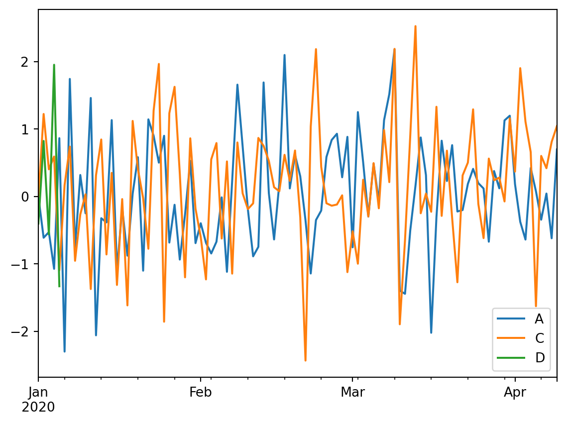
We can also combine operations before plotting the data using cumsum (cumulative sum) and then plot the data from there.
df3.cumsum().plot()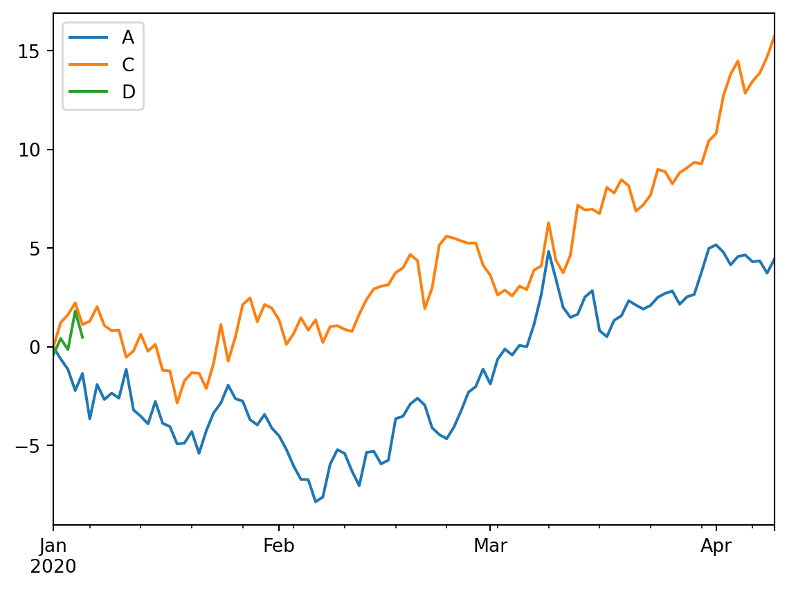
We can also make different kinds of plots, like this scatterplot for example.
df3.plot(kind='scatter', x='A',y='C')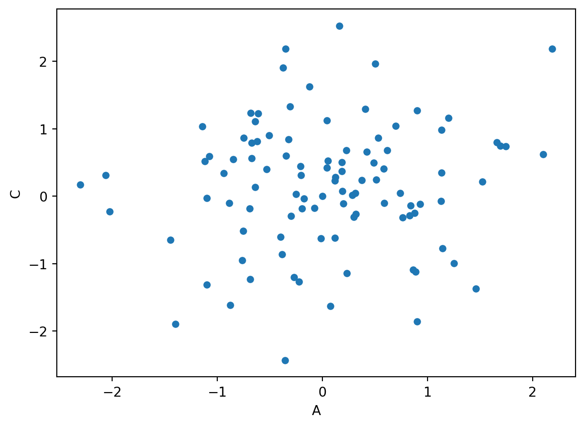
TipQuestion 9
Explore more options in the plot function, specifically altering the kind. Provide at least two relevant examples.
Working with categorical data
weekDays = pd.date_range(start='1/1/2020', periods=100, freq='D').strftime("%A")
df4 = pd.DataFrame({'Weekday':pd.Categorical(weekDays)}, columns=['Weekday'], index=pd.date_range(start='1/1/2020', periods=len(weekDays), freq='D'))
df5 = df3.join(df4)
We have now added a column with all the weekday. In the first line we transformed the datetime array to week names using the comment .strftime("%A"). You can use strftime for all kind of time conversation or rewriting options. You can explore https://strftime.org for options, they are also used in other programming languages. The pd.Categorical is used to enforce that Pandas sees the data as categorical. You can check this by using
df5.dtypesA float64
C float64
D float64
Weekday category
dtype: objectdf5.dropna().groupby("Weekday").mean()| A | C | D | |
|---|---|---|---|
| Weekday | |||
| Friday | -0.528172 | 0.403492 | -0.562305 |
| Saturday | -1.072969 | 0.593579 | 1.954878 |
| Sunday | 0.865408 | -1.094912 | -1.331952 |
| Thursday | -0.611756 | 1.224508 | 0.824006 |
| Wednesday | 0.000000 | 0.000000 | -0.400878 |
TipQuestion 10
Describe in your own words what you see after running the groupby(“Weekday”) command.
What you have learned today
If all is well you have learned today:
Explore data
Manipulating data
Dealing with missing values
Simple visuals
Working with categorical data