import pandas as pd
import matplotlib.pyplot as plt
from statsmodels.formula.api import ols
import numpy as npLinear regression 1: debunking sexual selection
Introduction
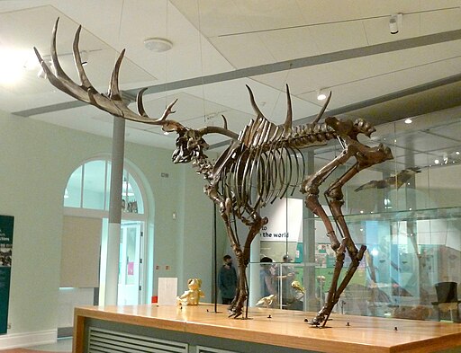
The Irish deer Megaloceros giganteus, formerly called the Irish elk, is one of the iconic members of the Ice Age fauna. Now extinct, it reached some 2.1 m shoulder height and it massive antlers spanned up to 3.6 m. In modern deer, large antlers and scary display of them predict a high success among females and thus a high reproductive success. This is an example of sexual selection, through which mating “decorations” or behaviors undergo positive selection, even though they may have no other use in one sex other than impressing its potential mating partners. This must have appealed to the Victorian prudery and the “survival of the sexiest”.
Linear regression is how you can tell whether this spicy explanation is correct, as has been done by the evolutionary biologist Steven J. Gould (1974). He measured the shoulder heights and antler lengths of deer species of various sizes and showed that they fell on a line that describes the relationship. The antler length for the Irish elk was exactly as predicted based on this relationship for smaller deer. Indeed, the Irish deer survived for tens of thousands of years with its giant antlers and fared well until the end of the Pleistocene. Like many animals of the Pleistocene megafauna, its extinction is attributed to climate change and hunting by early humans.
Can you replicate Gould’s landmark study?
Load and explore the data
Gould (1974) didn’t provide the dataset in his paper, which in 1974 is forgivable. His study was replicated by Plard et al. (2011) who included a dataset in an appendix. This dataset has been converted to csv for you.
antlers = pd.read_csv('../Data/Antler_allometry.csv')Preview the data:
antlers.head()Preview the bivariate distribution of the body mass and antler length:
fig, ax = plt.subplots()
ax.plot(antlers.Male_body_mass, antlers.Antler_length, '.')
ax.set_ylabel('Antler length [mm]')
ax.set_xlabel('Body mass [kg]')
This plot doesn’t look like a straight line, does it? The data is skewed and the apparent curve is not linear.
Many variables, such as those related to surface and volume, grow as powers of the linear dimensions, e.g. the body mass tends to grow as the cube of the body length. The exact scaling between the size of an organism and various biological variables is called the allometric constant and allometric power. In general, the relation between two biological quantities (like body size and antler length) is expressed using the allometric equation:
\(Y = a \cdot X^b\)
- Y is the biological variable of interest (e.g., metabolic rate).
- X is another biological measure, typically body size or mass.
- a is the allometric constant, also known as the proportionality constant.
- b is the allometric exponent or scaling exponent, which determines how the biological variable scales with size.
But this is a power law, and you want to apply linear regression. How to solve this? By using Gould’s (1974) original approach and transforming both the dependent and independent data using the natural logarithm \(\mathrm{ln}\) (using the log() function). This gives you the linear equation in the form:
\(\mathrm{ln}~Y = b_0 + b_1 \cdot{} \mathrm{ln}~X\)
which you can rewrite to:
\(Y = e^{b_0} X^{b_1}\)
Giving \(a = e^{b_0}\) and \(b = b_1\).
To perform the transformation, add two new columns to the data frame with the transformed variables:
antlers['Male_mass_ln'] = np.log(antlers.Male_body_mass)
antlers['Antler_length_ln'] = np.log(antlers.Antler_length)
Now plot the data again, using the transformed values
fig, ax = plt.subplots()
ax.plot(antlers.Male_mass_ln, antlers.Antler_length_ln, '.')
ax.set_ylabel('ln Antler length [mm]')
ax.set_xlabel('ln Body mass [kg]')
In this plot the log-transformed variables lie more or less along a line, to which you can fit a linear model using ordinary least-squares (OLS) regression.
Calculating regression coefficients using OLS
In the lecture, you learned that regression coefficients can be estimated by minimizing the sum of squares of the deviations between estimated values \(\hat{y}\) and observed values \(y_i\).
In practice, this means calculating the following system:
\(\bar{x} = \frac{\sum_{i=0}^{n} x_i}{n}\)
\(\bar{y} = \frac{\sum_{i=0}^{n} y_i}{n}\)
\(a = \bar{y} - b \cdot \bar{x}\)
\(b = \frac{\sum_{i=0}^{n} x_i y_i - \left(\sum_{i=0}^{n} x_i \sum_{i=0}^{n} y_i\right)/n}{\sum_{i=0}^{n} x^2_i - \left(\sum_{i=0}^{n} x_i \right)^2/n}\)
Although performing OLS regression is rarely done by hand, it is useful to do this once to understand what is happening in the simplest case. It is much easier to calculate in Python than truly by hand!
Try to use numpy and pandas to perform the above calculations in Python, using the antlers data frame.
Solution
Let n be the number of samples:
n = antlers.shape[0]To shorten the code and keep variable naming consistent with the equations above, let’s refer to the predictor variable (ln body mass) as x and the response variable (ln antler length) as y:
antlers['x'] = antlers.Male_mass_ln
antlers['y'] = antlers.Antler_length_ln
Sxx = np.sum(antlers.x**2) - np.sum(antlers.x)**2/n
Sxy = np.sum(antlers.x*antlers.y) - np.sum(antlers.x)*np.sum(antlers.y)/n
mean_x = np.mean(antlers.x)
mean_y = np.mean(antlers.y)The slope and intercept of the regression line are then:
b = Sxy / Sxx
a = mean_y - b * mean_x
Prediction
Using the determined equation, calculate the predicted value \(\hat{y}_i\) for each observation \(x_i\) and add it to antlers. Also, make the same scatter plot as before, now including the regression line you have calculated by “hand”.
Solution
antlers["fitted"] = a + b * antlers.xfig, ax = plt.subplots()
ax.plot(antlers.x, antlers.y, '.')
ax.plot(antlers.x, antlers.fitted, '-', color='#00000080')
ax.set_ylabel('ln Antler length [mm]')
ax.set_xlabel('ln Body mass [kg]')
TipQuestion 1
- What is the equation of the regression line?
- According to your linear model, what is the predicted antler length for an elk with a body mass of 160 kg?
Assessing the goodness of fit
The goodness of fit of a regression line is assessed using \(R^2\), the coefficient of determination. To determine \(R^2\), one compares the variation of the regression line around the mean value, i.e. the so-called sums of squares due to the model (\(\mathrm{SS_{mod}}\)) with the total variation in the dependent variable around its mean, i.e. the total sums of squares (\(\mathrm{SS_{tot}}\)). See this post on 365datascience.com for a visual explanation of the different sums of squares.
Using Python, calculate both of these sums of squares and \(R^2\) using:
\(\mathrm{SS_{mod}}={\sum_{i=1}^{n}\left({\hat{y}}_i-{\overline{y}}_i\right)^2}\)
\(\mathrm{SS_{tot}}={\sum_{i=1}^{n}\left({y_i}-{\overline{y}}_i\right)^2}\)
\(R^2=\frac{\mathrm{SS_{mod}}}{\mathrm{SS_{tot}}}\)
TipQuestion 2
- What values does the coefficient of determination take?
- What is the \(R^2\) value of the fitted model?
- Is this a good fit?
Running a regression function
Normally, you would use statistical software to calculate the results. This will not only get you the results faster, but also provide you with lots of useful additional information about the fit.
In Python, you can perform a regression using the statsmodels module. To fit a regression and show its results in the console, use the code below. This sets up an ordinary least square models object with Antler_length_ln as dependent (or endogenous) variable and Male_mass_ln as independent (or exogenous) variable, fits the regression, and performs several statistical tests on the model.
model     = ols("Antler_length_ln ~ Male_mass_ln", data=antlers)
model_fit = model.fit()
print(model_fit.summary2())
Do the results agree with your manual calculations?
When presenting results in a thesis or paper, it is always important to provide sufficient information about statistical results. Therefore, extract the attributes with the regression coefficients and the \(R^2\) value from model_fit and add them as annotation to the corner of the plot using plt.annotate(). Tip: check the help file for a statsmodels.regression.linear_model.RegressionResults object.
TipQuestion 3
Which attributes/properties of the model_fit object do you need for this?
You have now established a statistically-determined relation between body mass and antler length in deer, assessed how much of the variability in the dataset is represented, and plotted the results. In the next exercise you will look into statistically assessing the model results and testing the validity of the approach.
References
- Gould, S.J., 1974. The origin and function of “bizarre” structures: antler size and skull size in the “Irish Elk,” Megaloceros Giganteus. Evolution 28, 191–220. https://doi.org/10.1111/j.1558-5646.1974.tb00740.x
- Plard, F., Bonenfant, C., Gaillard, J.-M., 2011. Revisiting the allometry of antlers among deer species: male–male sexual competition as a driver. Oikos 120, 601–606. https://doi.org/10.1111/j.1600-0706.2010.18934.x