import random
import numpy as np
import matplotlib.pyplot as plt
import statsmodels.api as sm
from statsmodels.tsa.stattools import acf, pacf
from statsmodels.graphics.tsaplots import plot_acf, plot_pacf
from statsmodels.tsa.arima_process import ArmaProcess
from scipy import statsAutoregressive processes
Before we analyze some real-life datasets, let’s first fabricate some. Why fabricate data? This is the principle of simulations, which we often use to e.g. to test if our idea of how something works (= our model) gives the same results as we see in real life. So to check if a test or a regression model describes a relationship correctly, we might want to simulate a process with known parameters and check how well it is recovered by the regression model we fit.
A second motivation is to give you an intuition as to what common types of processes in geosciences are. We will look at the simplest stochastic process, a random walk, and a simple autoregressive process, also known as the red noise. Their manifestations can look deceivingly similar in a time series plot, but they have very different properties.
What causes autocorrelation?
To understand what an autoregressive process is, let’s first consider a simple example: a random walk.
Random walk is a stochastic process where the next value is determined by the previous value plus a random increment. This is a very simple model of a process that is not stationary, and it is often used as a null hypothesis in many tests, also in geosciences.
TipQuestion 1
Can you write your own code for a random walk process in one dimension?
Hint
If you don’t know how to start, try to write it as pseudocode: human words describing step by step (in an algorithm) values, where each subsequent value increases by 1 or decreases by 1 with equal probabilities. Submit the pseudocode as your answer. Then you can translate it into python step by step. We will appreciate code that may not even fully work but where we can see that you tried on your own.
Python operators+= and -= may be useful!
The code in the answer to question 1 is useful to understand how the random walk is generated. But steps in a random walk don’t always have to be of length 1, their lengths can have a normal distribution. We can draw values from a normal distribution using the numpy function random.normal().
np.random.seed(123)
y = np.cumsum(np.random.normal(loc=0, scale=1, size=1000))
plt.plot(y[1:500])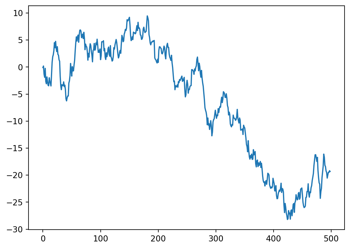
This of course looks like a strong trend. If this was diversity, we would say “mass extinction”. If this was temperature, we would be back to a Snowball Earth. Is this really a random walk? Let’s plot the rest of it.
plt.plot(y[500:1000])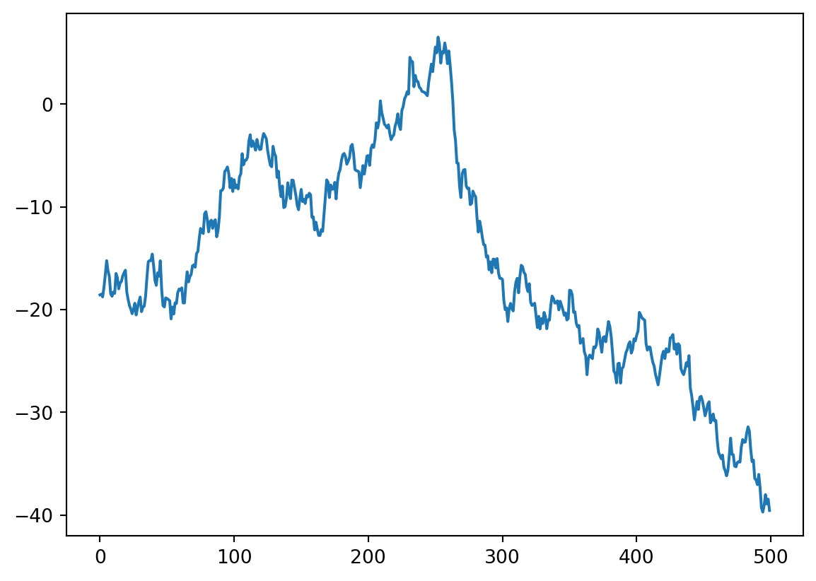
It even has regular-looking zig-zaggy peaks that make it look as if there was some periodicity in this process. This gives you an idea how easy it is to see patterns in random wiggles. That’s why we need statistical models to tell us if a process is anything different from random noise. So how can we characterize noise in a time series?
Autocorrelation function
plot_acf(y)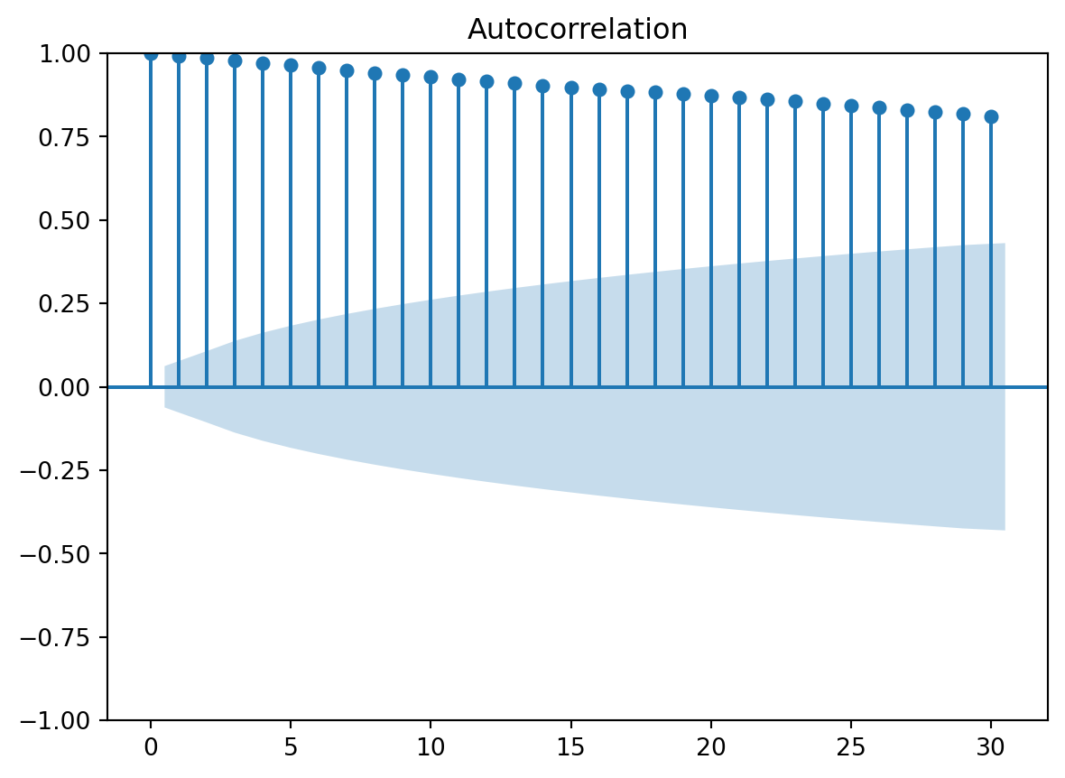

This plot shows you that a random walk is strongly autocorrelated. We can extract the values of autocorrelation at different lags using the acf function:
acf(y)array([1. , 0.99285668, 0.98567537, 0.97838588, 0.9712757 ,
0.96380735, 0.955839 , 0.94856451, 0.94162449, 0.93505323,
0.92842868, 0.92179431, 0.91530125, 0.90930533, 0.90310993,
0.89737722, 0.89234135, 0.88735087, 0.88252776, 0.87716526,
0.87200085, 0.86664339, 0.8610253 , 0.8551481 , 0.84900706,
0.84300438, 0.83698006, 0.83048987, 0.82417489, 0.81761755,
0.81157364])The first number is always 1: this is the zero-lag coefficient, i.e. coefficient fo correlation of each value with itself.
Autoregressive processes
An autoregressive process is usually just part of a more complex empirical time series. But we need to understand and isolate it to decompose an empirical time series into its components.
The simplest autoregressive process is of order 1, also written AR(1), and can be modeled as \(X_t = \beta + \alpha X_{t-1} + \epsilon_t\).
This is also known as the “red noise” and is very important in many modeling applications. For example, you will encounter it in cyclostratigraphy (as the null hypothesis in testing for astronomical forcing) or in paleobiology when studying trait evolution in the absence of selection (aka “genetic drift”).
We can generate autoregressive processes with various parameters using the tsa module in statsmodels. The function ArmaProcess stands for “AutoRegressive Moving Average”, but now we are only interested in the autoregressive part so we can ignore the Moving Average part. By setting the zero-lag coefficient of the MA process to 1 we make it basically absent.
The parameters of an AR process will be 1 (order) and \(\alpha\). Because of conventions in the field of signal processing, the sign of \(\alpha\) has to be flipped. For example, for an AR(1) process with \(\alpha = 0.5\), the array representing the AR parameters would be ar = np.array([1, -0.5]).
ar1 = np.array([1, -0.5])
ma1 = np.array([1])
AR_object = ArmaProcess(ar1, ma1)
simulated_data = AR_object.generate_sample(nsample=1000)
plt.plot(simulated_data)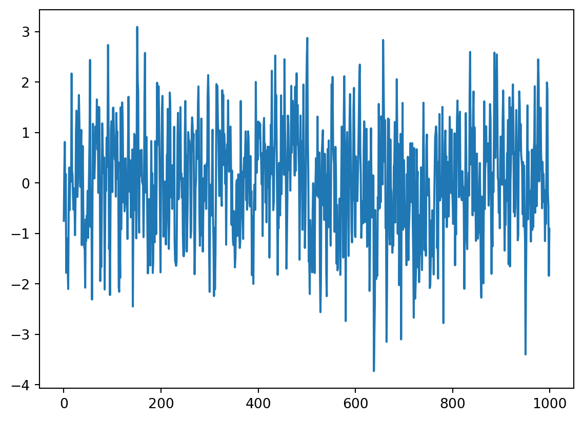
Make your own AR processes
To gain an intuition of the behavior of an AR process, try to write code and plot AR processes with different processes by modifying the example above. Make an acf plot for each of the processes to check if you solved it correctly. Many solutions are possible.
TipQuestion 2
How do you simulate a process where the strongest correlation is at lag 2? Remember that this is described by AR-coefficients \(\alpha_k\), for k = 1, 2,…, p
TipQuestion 3
How do you simulate a process with negative autocorrelation (also called a “repulsive” process)?
Putting regression into autoregression
In the previous steps you have created the variable y, which is a random walk and thus an AR(1) process. Autoregressive means that each value \(y_i\) can be predicted not by a different variable (“predictor” or “independent variable”), but by the previous value \(y_{i-1}\). So you can use the i - 1 value to predict the ith value.
To do this, you need to create a second, dummy variable that is the the i - 1 value of y. In numpy, you can use the roll() function to create a new variable that is the the i - 1 value of the trend.
z = np.roll(y, -1)
TipQuestion 4
What is the slope coefficient of a linear regression model of y over z (i.e. of \(y_i\) over \(y_{i-1}\))? And what is the goodness of fit?
Hint
Last week you used statsmodels ols() function because both variables were in the same pandas dataframe. You would need to join y and z into one dataframe (good pandas practice!) or you need to use the OLS() function of statsmodels, which allows regression over separate numpy arrays.
Testing for autocorrelation
Last week you learned how to use the Durbin-Watson test. This test is based on the residuals of the regression of \(X_t\) on \(X_{t-1}\). Examine the output of the regression model you fitted in question 4.
TipQuestion 5
What is the conclusion of the Durbin-Watson test for autocorrelation in your regression model for the random walk over itself?
Hint
You may need to add an import of the relevant test fromstatsmodels and need a table with critical values for larger samples, for example: https://real-statistics.com/statistics-tables/durbin-watson-table/
Partial autocorrelation function (PACF)
Partial correlation, in general, is the correlation between two variables after removing the effect of other variable(s). In time series, this is the correlation between \(X_t\) and \(X_{t-k}\) after removing the effect of \(X_{t-1}, X_{t-2}, ..., X_{t-k+1}\). In practice, we use the partial autocorrelation function to identify the order of an autoregressive process. The order is equal to the number of “lollipops” that stick out from the blue shaded area. You can create a PACF plot using plot_pacf() and see the correlation coefficients using the pacf() functions. Mind the imports!
TipQuestion 6
What would you detect as the order of the random walk you generated?
TipQuestion 7
Earlier in this practical, you created an AR(2) process saved under the name simulated_data_2. Can you correctly recover the order of the process from a PACF plot?
If you examine the correlation coefficients in the answers to the last two questions, you will realize it is relatively easy to identify the order of the process. But recovering the \(\alpha\) coefficient(s) is much harder. We don’t have a simple function to do this: like in any other regression analysis, we have to fit models to find the parameters of an AR process. We will do this in the second practical.