import pandas as pd
import matplotlib.pyplot as plt
import seaborn as sns
import statsmodels.api as sm
from statsmodels.formula.api import ols
from statsmodels.stats.diagnostic import het_breuschpagan
import numpy as np
import scipy.stats as stats
# read data
antlers = pd.read_csv('../Data/Antler_allometry.csv')
# apply natural log transform to the key variables
antlers['Male_mass_ln'] = np.log(antlers.Male_body_mass)
antlers['Antler_length_ln'] = np.log(antlers.Antler_length)
# sort dataframe along our desired x-axis for easier plotting of lines
antlers = antlers.sort_values("Male_mass_ln")
# rename sub family column
antlers = antlers.rename(columns={'Sub-family':"sub_fam"})
# make scatterplot of the transformed data
fig, ax = plt.subplots()
ax.plot(antlers.Male_mass_ln, antlers.Antler_length_ln, '.', color='k')
ax.set_ylabel('ln Antler length [mm]')
ax.set_xlabel('ln Body mass [kg]')
# run regression using python
model = ols("Antler_length_ln ~ Male_mass_ln", data=antlers)
model_fit = model.fit()Linear regression 2: debunking sexual selection
Introduction
Goal of today’s exercise
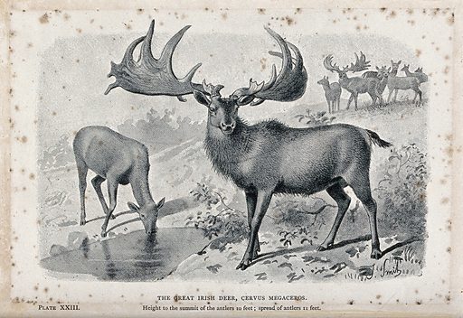
In the previous exercise, you have transformed the data set of antler lengths for the Irish elk (Plard et al., 2011) to remove skew from the distribution using a natural logarithm, calculated the regression line, and assessed the goodness of fit. But how good is the fit really? Was linear regression a valid approach to use for these data? Can we statistically answer the question: is deer body mass related to antler length?
Today, you’ll try to find the answers to these questions.

Parametric statistics
Parametric techniques are statistical methods that assume a specific form for the underlying population distribution. These methods often rely on population parameters (such as means and variances) that summarize the data and make certain assumptions about their structure. Linear regression is also a parametric technique, because it makes specific assumptions about the form of the relationship between the dependent and independent variables. Specifically, it assumes that this relationship can be described using a linear equation of the form:
\(y=\beta_0 + \beta_{1}x_{1}+\epsilon\)
Here, \(\beta_0\) and \(\beta_1\) are the parameters of the model, and \(\epsilon\) represents the error term. The parametric nature of linear regression means that once we estimate these population parameters from the sample data by calculating regression coefficients \(b_0\) and \(b_1\), we can use them to make predictions and perform further analysis based on the underlying assumptions of the data distribution. Particularly the assumptions about the normal distribution of the errors at any point along the x-scale is important. This means we can apply the statistical tests that are related to the normal distribution founded in the Central Limit Theorem, such as the t-test and F-test (also see Chapter 6.3–6.4 of Haslwanter, 2022).
Setup, load data, and fit regression model
Use the following code to load the data of the previous exercise and fit the regression model using ordinary least squares (OLS):

Task 1: Statistical testing in linear regression
Statistical testing (in linear regression) is all about making informed decisions based on data by systematically evaluating hypotheses, similar to other testing procedures in statistics. The core steps to follow are:
- State null and alternative hypotheses
- Choose significance level
- Select the appropriate test
- Compute test statistic using data
- Determine p-value and/or critical value for test statistic
- Make a decision on the hypothesis
Follow the above steps using the antler dataset and the model_fit to find out whether there is a statistically significant relation between antler length and male body mass. Use the two tests for this that apply to linear regression: the t-test and F-test. Follow the tips below for more information on how to perform this, refer to lecture slides on linear regression, the statsmodels package user guide, the text book (Haslwanter, 2022), and other online sources.
T-test
A t-test is used to determine whether a specific coefficient (\(\beta_i\)) is significantly different from zero. In other words, it helps to assess whether an independent variable has a meaningful impact on the dependent variable. The t-test compares the estimated coefficient to its standard error, providing a p-value that indicates the likelihood of observing such a result by chance.
You can run a t-test on the model fit simply by showing the model summary in the console.
# Perform t-test using the summary2()
print(model_fit.summary2()) Results: Ordinary least squares
=================================================================
Model: OLS Adj. R-squared: 0.801
Dependent Variable: Antler_length_ln AIC: 50.0742
Date: 2026-03-06 15:57 BIC: 52.9421
No. Observations: 31 Log-Likelihood: -23.037
Df Model: 1 F-statistic: 121.9
Df Residuals: 29 Prob (F-statistic): 6.68e-12
R-squared: 0.808 Scale: 0.27667
------------------------------------------------------------------
Coef. Std.Err. t P>|t| [0.025 0.975]
------------------------------------------------------------------
Intercept 1.6811 0.3838 4.3803 0.0001 0.8962 2.4661
Male_mass_ln 0.9904 0.0897 11.0396 0.0000 0.8069 1.1739
-----------------------------------------------------------------
Omnibus: 4.515 Durbin-Watson: 1.522
Prob(Omnibus): 0.105 Jarque-Bera (JB): 3.444
Skew: -0.812 Prob(JB): 0.179
Kurtosis: 3.167 Condition No.: 18
=================================================================
Notes:
[1] Standard Errors assume that the covariance matrix of the
errors is correctly specified.
- Formulate \(H_0\) and \(H_A\) for a t-test of \(\beta{}_{1}\)
- Is the t-test in this case one-sided or two-sided? Briefly explain why.
- What is the test statistic value for \(\beta{}_{1}\)?
- What is the critical t value at alpha=0.05 (tip: use
scipy.stats.t.isf())?
- What is your decision on the formulated hypotheses?
- If testing for any relation between the two variables (the default case in regression):
\(H_0: \beta{}_{1} = 0\)
\(H_A: \beta{}_{1} \neq 0\)
If only testing for on positive relation between mass and length:
\(H_0: \beta{}_{1} = 0\)
\(H_A: \beta{}_{1} > 0\)
- In the first hypothesis case, it is a two sided test. The slope can either be positive or negative. In the second case, it is a one sided test, since we’re only focusing on a positive slope result.
- The t-value for \(\beta{}_{1}\) is listed in the summary table, and equals 11.0396.
stats.t.isf(0.05/2, 29)gives \(t_{\mathrm{critical}} = 2.045\). This is for a two-sided test (\(\alpha/2\)) and \(n-2\) degrees of freedom.
- The test statistic is much larger than the critical value, so \(H_0\) is rejected. There is a significant relation between body mass and antler length.
ANOVA and F-test
The F-test evaluates the overall significance of the regression model. It tests whether at least one of the coefficients is different from zero, indicating that the model provides a better fit to the data than a model with no predictors. The F-test compares the explained variance of the model to the unexplained variance, yielding an F-statistic and a corresponding p-value.
Run an ANOVA on the linear regression fit to perform the F-test and inspect the results. Tip: use anova_lm().
# Perform F-test using anova function
print(sm.stats.anova_lm(model_fit)) df sum_sq mean_sq F PR(>F)
Male_mass_ln 1.0 33.718530 33.718530 121.871797 6.683873e-12
Residual 29.0 8.023492 0.276672 NaN NaN
Note that the F statistic and p-value is also provided by summary2()!
- Formulate \(H_0\) and \(H_A\) for an F-test of the regression
- What is the Mean Square Error (or \(\mathrm{MS_{res}}\)) for this model?
- Is the F-test one-sided or two-sided? Briefly explain why.
- What is p-value associated to the F-statistic in this case? What do you conclude from this?
- Compare this p-value to the p-value of the t-test of \(\beta{}_{1}\) (accessible using
model_fit.pvalues). What do you notice? How can this be?
- \(H_0: \beta{}_{1} = \beta{}_{2} = ... = \beta{}_{n} = 0\)
\(H_A:\) At least one \(\beta{}_{i} \neq 0\)
- MSE is 0.276672
- The F test is a one-sided test, since it compares whether a ratio between two variances falls in extreme range of the F-distribution.
- The p-value is \(6.68 \times 10^{-12}\). This is much lower than alpha and we can reject \(H_0\).
- The p-value is identical to the one for the t-test. This is due to the F-test only testing \(\beta{}_{1} = 0\) in this case of simple linear regression, since there is only one independent variable. This is the same hypothesis for the t-test performed above. In multiple regression, the p-values will be different between the two tests.
Task 2: Estimating confidence intervals and belts
Confidence intervals are used to estimate the range within which a population parameter is likely to lie, based on sample data. They provide a measure of uncertainty around a point estimate with a given confidence level (\(\alpha\)). The model_fit summary provides the 95% confidence intervals of both \(\beta_0\) and \(\beta_1\).
Additionally, a confidence belt of the model fit can also be constructed, which shows where the real population mean of \(\hat{y}_i\) would lie (with \(\alpha\) confidence). Such confidence belts are often displayed on plots with regression lines. Calculate the confidence belt for the fit by using the subroutine .get_prediction() on the model_fit object, and subsequently the .summary_frame() subroutine on the prediction object.
Plot the log-transformed data again, include the regression line, annotate it with the regression equation, \(R^2\) value, p-value, and add the lower and upper limits of the confidence belt to the plot as shading. Tip: use .fill_between to create shading between two lines.
The data frame returned by .summary_frame() also provides the confidence interval for the observations, the so-called prediction interval. Add it to the plot and compare its values with the confidence interval for the mean.
Check confidence interval of the coefficients in the summary table. Shown as last two columns under the header [0.025 0.975]:
print(model_fit.summary2()) Results: Ordinary least squares
=================================================================
Model: OLS Adj. R-squared: 0.801
Dependent Variable: Antler_length_ln AIC: 50.0742
Date: 2026-03-06 15:57 BIC: 52.9421
No. Observations: 31 Log-Likelihood: -23.037
Df Model: 1 F-statistic: 121.9
Df Residuals: 29 Prob (F-statistic): 6.68e-12
R-squared: 0.808 Scale: 0.27667
------------------------------------------------------------------
Coef. Std.Err. t P>|t| [0.025 0.975]
------------------------------------------------------------------
Intercept 1.6811 0.3838 4.3803 0.0001 0.8962 2.4661
Male_mass_ln 0.9904 0.0897 11.0396 0.0000 0.8069 1.1739
-----------------------------------------------------------------
Omnibus: 4.515 Durbin-Watson: 1.522
Prob(Omnibus): 0.105 Jarque-Bera (JB): 3.444
Skew: -0.812 Prob(JB): 0.179
Kurtosis: 3.167 Condition No.: 18
=================================================================
Notes:
[1] Standard Errors assume that the covariance matrix of the
errors is correctly specified.
Get confidence belt for the fit:
model_pred = model_fit.get_prediction()
pred_summary = model_pred.summary_frame(alpha=0.05)
pred_summary| mean | mean_se | mean_ci_lower | mean_ci_upper | obs_ci_lower | obs_ci_upper | |
|---|---|---|---|---|---|---|
| 17 | 4.142143 | 0.176472 | 3.781218 | 4.503068 | 3.007429 | 5.276858 |
| 29 | 4.221416 | 0.170450 | 3.872807 | 4.570025 | 3.090559 | 5.352273 |
| 18 | 4.258794 | 0.167642 | 3.915927 | 4.601660 | 3.129694 | 5.387894 |
| 12 | 4.543709 | 0.147043 | 4.242973 | 4.844445 | 3.426681 | 5.660737 |
| 25 | 4.543709 | 0.147043 | 4.242973 | 4.844445 | 3.426681 | 5.660737 |
| 16 | 4.597256 | 0.143360 | 4.304053 | 4.890460 | 3.482233 | 5.712280 |
| 15 | 4.696377 | 0.136734 | 4.416724 | 4.976031 | 3.584840 | 5.807915 |
| 14 | 4.786474 | 0.130956 | 4.518640 | 5.054309 | 3.677851 | 5.895097 |
| 24 | 4.849046 | 0.127096 | 4.589104 | 5.108987 | 3.742303 | 5.955788 |
| 21 | 4.981293 | 0.119415 | 4.737061 | 5.225525 | 3.878134 | 6.084452 |
| 28 | 5.158909 | 0.110311 | 4.933298 | 5.384520 | 4.059723 | 6.258095 |
| 1 | 5.358993 | 0.102140 | 5.150094 | 5.567893 | 4.263115 | 6.454871 |
| 22 | 5.382859 | 0.101338 | 5.175600 | 5.590118 | 4.287292 | 6.478425 |
| 13 | 5.451188 | 0.099266 | 5.248166 | 5.654210 | 4.356415 | 6.545961 |
| 7 | 5.594379 | 0.096080 | 5.397873 | 5.790885 | 4.500796 | 6.687962 |
| 10 | 5.845391 | 0.094616 | 5.651878 | 6.038903 | 4.752341 | 6.938440 |
| 0 | 6.132152 | 0.099493 | 5.928667 | 6.335638 | 5.037293 | 7.227011 |
| 23 | 6.191217 | 0.101298 | 5.984039 | 6.398395 | 5.095666 | 7.286768 |
| 8 | 6.196416 | 0.101469 | 5.988888 | 6.403944 | 5.100799 | 7.292033 |
| 6 | 6.290338 | 0.104873 | 6.075848 | 6.504828 | 5.193381 | 7.387295 |
| 30 | 6.304386 | 0.105432 | 6.088753 | 6.520019 | 5.207205 | 7.401568 |
| 26 | 6.358667 | 0.107705 | 6.138385 | 6.578950 | 5.260563 | 7.456772 |
| 20 | 6.501858 | 0.114501 | 6.267677 | 6.736039 | 5.400881 | 7.602835 |
| 27 | 6.672857 | 0.123914 | 6.419425 | 6.926290 | 5.567625 | 7.778089 |
| 9 | 6.888069 | 0.137336 | 6.607186 | 7.168952 | 5.776221 | 7.999917 |
| 2 | 6.948111 | 0.141333 | 6.659053 | 7.237169 | 5.834170 | 8.062052 |
| 11 | 6.995506 | 0.144555 | 6.699859 | 7.291154 | 5.879838 | 8.111175 |
| 4 | 7.092421 | 0.151308 | 6.782962 | 7.401881 | 5.973013 | 8.211829 |
| 5 | 7.149496 | 0.155380 | 6.831708 | 7.467284 | 6.027757 | 8.271235 |
| 3 | 7.482733 | 0.180282 | 7.114014 | 7.851451 | 6.345516 | 8.619950 |
| 19 | 7.800693 | 0.205368 | 7.380668 | 8.220718 | 6.645820 | 8.955566 |
Put everything together in a plot:
# get values from model fit objects
intercept = model_fit.params.iloc[0]
slope = model_fit.params.iloc[1]
rsquared = model_fit.rsquared
p_value = model_fit.pvalues.iloc[1]
# construct the label, rounding numbers
label = f'y = {intercept:.2f} + {slope:.2f}x\np = {p_value:0.2E}\nR2 = {rsquared:0.2f}'
# create figure
fig, ax = plt.subplots()
ax.set_ylim(2.6,9.4)
# add (axes) labels
ax.set_ylabel('ln Antler length [mm]')
ax.set_xlabel('ln Body mass [kg]')
plt.annotate(label, xy=(0.97, 0.03), xycoords='axes fraction',
fontsize=10, backgroundcolor='white',
horizontalalignment='right', verticalalignment="bottom")
# add data
ax.fill_between(antlers["Male_mass_ln"], pred_summary['obs_ci_lower'], pred_summary['obs_ci_upper'],
color='gray', alpha=0.25, edgecolor=None)
ax.fill_between(antlers["Male_mass_ln"], pred_summary['mean_ci_lower'], pred_summary['mean_ci_upper'],
color='gray', alpha=0.4, edgecolor=None)
ax.plot(antlers["Male_mass_ln"], model_fit.fittedvalues, '-', color='r', alpha=0.5)
ax.plot(antlers.Male_mass_ln, antlers.Antler_length_ln, '.', color='k')
- What would it mean if the lower confidence level of \(\beta_1\) would be below zero in this case? And what if confidence interval for \(\beta_0\) would encompass zero?
- What would be the likely effect of adding more data points on the confidence intervals? Why is that?
- Why is the prediction interval wider than the confidence interval?
- If the lower confidence limit of slope \(b_1\) would include 0, it means that there is a likelihood within alpha that the real population slope is 0. This would result in acceptance of \(H_0\) in a t-test and a statistically insignificant slope. For the intercept \(b_0\) this does not matter, since that can fall below zero and does not impact the relation between the variables.
- If data points fall within the normal range of the existing data, it would tighten the confidence intervals, since they are based on the standard error which has n in the denominator. More points in same range = more certainty that signal is the true population signal.
- The prediction interval includes not only the uncertainty in estimating the mean response (as the confidence interval does) but also the inherent variability (randomness) of the individual observations around that mean. This results in more uncertainty.
Task 3: Assessing validity of a linear model
A final crucial aspect of hypothesis testing is verifying that the assumptions of the statistical methods used are valid. For hypothesis tests related to linear regression to be reliable, the model’s underlying assumptions (linearity, normality of errors, homoscedasticity, and independence of errors) must be satisfied. If these assumptions are not met, the results of the hypothesis tests may be compromised. This could for instance mean that the calculations of test statistics and p-values are inflated and statistical significance is wrongfully inferred.
Using the antler data and the fitted linear model, test whether the each of the above assumptions of linear regression are met.
Linearity
Check if the relationship between the independent and dependent variables is linear.
- Plot the observed values of the dependent variable against the independent variable(s). Look for a linear pattern (straight line) rather than a curve or other non-linear patterns.
- Plot the residuals against the independent variable. For linearity, there should be no obvious patterns (e.g., curves or systematic structures). The residuals can be calculated by \(y_i-\hat{y}_i\), or taken from the
model_fitobject.
# make scatterplot of the transformed data
fig, ax = plt.subplots()
ax.set_ylabel('ln Antler length [mm]')
ax.set_xlabel('ln Body mass [kg]')
ax.plot(antlers.Male_mass_ln, antlers.Antler_length_ln, '.')
# make residual plot
fig, ax = plt.subplots()
ax.set_xlabel('x')
ax.set_ylabel(r'$y-\hat{y}$')
ax.set_ylim(-0.8,0.8)
ax.axhline(y=0.0, color='black', linestyle='--', linewidth=1)
ax.plot(antlers.Male_mass_ln, model_fit.resid, '.')
Do you think the linearity assumption is met? Why?
There appears to be an inherent curve in the data, parabola shaped, which is even clearer in the residual plot. Is is not only a few values in the outside range along the x axis, so linearity might be an issue.
Normality
To test for normality of the residuals/error, there are a few approaches possible. Try the following:
- Make a histogram of the residuals and assess its shape.
- Plot the quantiles of the residuals against the quantiles of a normal distribution, this is a so-called Q-Q plot. The points should roughly fall along a straight line 1:1 if the residuals are normally distributed. Tip: use
sm.qqplot()for this. - Apply a proper statistical test to assess normality. You can use the Shapiro-Wilk test for this using \(\alpha = 0.05\) (tip: use
scipy.stats.shapiro()).
# make a histogram
fig = plt.hist(model_fit.resid)
plt.show()
# make qqplot
fig = sm.qqplot(model_fit.resid, line='45')
plt.show()
# apply shapiro test
stats.shapiro(model_fit.resid)ShapiroResult(statistic=np.float64(0.9191887179783036), pvalue=np.float64(0.02246587309516523))
Do you think the normality of errors assumption is met? Why?
Both the histogram and the QQ-plot show that there is not really a normal distribution of the residuals This is confirmed by the Shapiro-Wilk test, which results in a p-value of 0.02, this means rejecting \(H_0\).
\(H_0:\) The data are normally distributed.
Homoscedasticity
To check if the residuals have constant variance (homoscedasticity) across all levels of the independent variable:
- Plot the residuals against the independent variable and assess the shape.
- Plot the absolute residuals against the independent variable and assess the shape. Now run a linear model in the form
abs_residuals ~ Male_mass_ln. Does this have a significant slope? - Run a Breusch-Pagan Test on the model using
het_breuschpagan(). As input you can usemodel_fit.resid(residuals of fitted model) andmodel.exog(independent data that was used for the OLS model). This test uses the following hypotheses:- \(H_0\): Homoscedasticity is present
- \(H_A\): Homoscedasticity is not present
# make residual plot
fig, ax = plt.subplots()
ax.set_xlabel('x')
ax.set_ylabel(r'$y-\hat{y}$')
ax.set_ylim(-0.8,0.8)
ax.axhline(y=0.0, color='black', linestyle='--', linewidth=1)
ax.plot(antlers.Male_mass_ln, model_fit.resid, '.')
# run regression on abs residuals
antlers['resid_abs'] = np.abs(model_fit.resid)
res_mod = ols("resid_abs ~ Male_mass_ln", data=antlers)
res_fit = res_mod.fit()
# make abs residual plot, add regression line
fig, ax = plt.subplots()
ax.set_xlabel('x')
ax.set_ylabel(r'$\vert{}y-\hat{y}\vert{}$')
ax.set_ylim(-0.05,0.75)
ax.plot(antlers.Male_mass_ln, np.abs(model_fit.resid), '.')
ax.plot(antlers.Male_mass_ln, res_fit.fittedvalues, '-')
# check summary of regression of abs residuals
print(res_fit.summary2()) Results: Ordinary least squares
=================================================================
Model: OLS Adj. R-squared: 0.027
Dependent Variable: resid_abs AIC: 13.7740
Date: 2026-03-06 15:57 BIC: 16.6420
No. Observations: 31 Log-Likelihood: -4.8870
Df Model: 1 F-statistic: 1.845
Df Residuals: 29 Prob (F-statistic): 0.185
R-squared: 0.060 Scale: 0.085786
------------------------------------------------------------------
Coef. Std.Err. t P>|t| [0.025 0.975]
------------------------------------------------------------------
Intercept 0.6978 0.2137 3.2654 0.0028 0.2608 1.1349
Male_mass_ln -0.0679 0.0500 -1.3583 0.1848 -0.1700 0.0343
-----------------------------------------------------------------
Omnibus: 8.643 Durbin-Watson: 2.432
Prob(Omnibus): 0.013 Jarque-Bera (JB): 7.227
Skew: 0.930 Prob(JB): 0.027
Kurtosis: 4.462 Condition No.: 18
=================================================================
Notes:
[1] Standard Errors assume that the covariance matrix of the
errors is correctly specified.
# run Breusch-Pagan Test
sm.stats.diagnostic.het_breuschpagan(model_fit.resid, model.exog)(np.float64(2.776325864505093),
np.float64(0.09566740664798264),
np.float64(2.8526920231619197),
np.float64(0.10194680406595764))
Do you think the model is homoscedastic? Why?
The regresssion fitted through the absolute residuals is not significant at \(\alpha = 0.05\) with \(p=0.185\). Also, the Breusch-Pagan test is not significant at \(\alpha = 0.05\) with \(p=0.096\), which means we accept \(H_0\) for this test.
\(H_0:\) Homoscedasticity is present
Independence / autocorrelation
Lack of independence of residuals/errors are an issue in linear regression. This often happens in time series data, where the value of an error term is correlated with the value of previous error terms (temporal autocorrelation), or sometimes when data are collected in space, e.g. in a single borehole or near each other in a certain x-y domain (spatial autocorrelation). Since the data in this study do not have these issues, we could skip this step for now. The steps are easy, however, and for the sake of learning to test for autocorrelation of residuals, confirm that it is absent.
To statistically test for autocorrelation (\(\rho\)) in linear regression, you use the Durbin-Watson test statistic \(d\) (see also 12.4c of Haslwanter, T., 2022.), which is simply provided by model_fit.summary2(). The values for \(d\) can range from 0 to 4, meaning:
- \(d=0\): perfect positive autocorrelation
- \(d=2\): no autocorrelation
- \(d=4\): Perfect negative autocorrelation
As a general guideline, Durbin-Watson test statistic values between 1.5 and 2.5 are considered acceptable. Values outside this range may indicate potential issues. Specifically, values below 1 or above 3 are definite causes for concern. If you want to be exact you have to look up (page 6) the critical lower (\(d_L\)) and upper (\(d_U\)) thresholds of the Durbin-Watson test statistic for a confidence level \(\alpha\) and specific combination of n (sample size, here 31) and k (number of independent variables in the model, here 1).
To statistically test for positive autocorrelation:
- If \(d < d_L\), there is statistical evidence that the error terms are autocorrelated
- If \(d > d_U\), there is no statistical evidence that the error terms are autocorrelated
- If \(d_L < d < d_U\), the test is inconclusive.
To statistically test for negative autocorrelation:
- If \((4-d) < d_L\), there is statistical evidence that the error terms are autocorrelated
- If \((4-d) > d_U\), there is no statistical evidence that the error terms are autocorrelated
- If \(d_L < (4-d) < d_U\), the test is inconclusive.
# get Durbin-Watson statistic in model summary
print(model_fit.summary2()) Results: Ordinary least squares
=================================================================
Model: OLS Adj. R-squared: 0.801
Dependent Variable: Antler_length_ln AIC: 50.0742
Date: 2026-03-06 15:57 BIC: 52.9421
No. Observations: 31 Log-Likelihood: -23.037
Df Model: 1 F-statistic: 121.9
Df Residuals: 29 Prob (F-statistic): 6.68e-12
R-squared: 0.808 Scale: 0.27667
------------------------------------------------------------------
Coef. Std.Err. t P>|t| [0.025 0.975]
------------------------------------------------------------------
Intercept 1.6811 0.3838 4.3803 0.0001 0.8962 2.4661
Male_mass_ln 0.9904 0.0897 11.0396 0.0000 0.8069 1.1739
-----------------------------------------------------------------
Omnibus: 4.515 Durbin-Watson: 1.522
Prob(Omnibus): 0.105 Jarque-Bera (JB): 3.444
Skew: -0.812 Prob(JB): 0.179
Kurtosis: 3.167 Condition No.: 18
=================================================================
Notes:
[1] Standard Errors assume that the covariance matrix of the
errors is correctly specified.
# combine DW statistic from summary2 and the limits taken from the online table
d = 1.483
dL = 1.363
dU = 1.496
if dL < d and d < dU:
print("DW test is inconclusive")DW test is inconclusive
The test is inconclusive, but theoretically there should be no autocorrelation in these data. How can this be?
There seem to be issues with linearity of the fit, which can give a fake sense of autocorrelation in the residuals of the regression. Before testing autocorrelation, one should first make sure the model used is appropriate.
Combining the results of the tests you performed on the regression result, answer the following question.
Are the assumptions of linear regression met sufficiently to validate the use of linear regression?
From the tests, we conclude that there is no clear linearity and the residuals are not normally distributed, but there is homoscedasticity. Two core assumptions are not met, and therefore we can conclude that linear regression is not an appropriate method for these data.
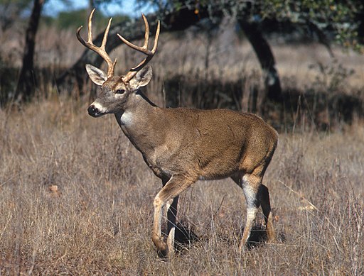
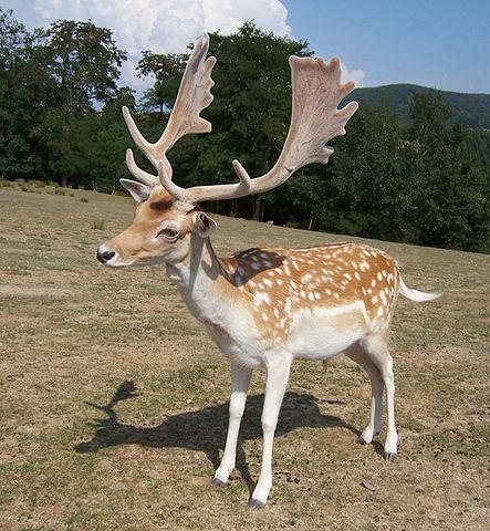
Task 4: Revisiting deer
One reason for the invalidity of the model could be the interplay between other independent variables that may be significantly controlling antler length and are not taken into account in your current model. For example, in the dataset by Plard et al. (2011) there are three sub families of deer, which may scale differently (Tsuboi et al., 2022): Muntiacinae (Muntjacs), Odocoileinae (“New World Deer”) and Cervinae (“Old World Deer”). Some examples of different species in these three sub families are shown below.
_male_head.jpg)


You can easily display the different sub-families in a plot using the seaborn plotting engine:
sns.scatterplot(
x = "Male_mass_ln",
y = "Antler_length_ln",
hue = "sub_fam",
style = "sub_fam",
data = antlers)
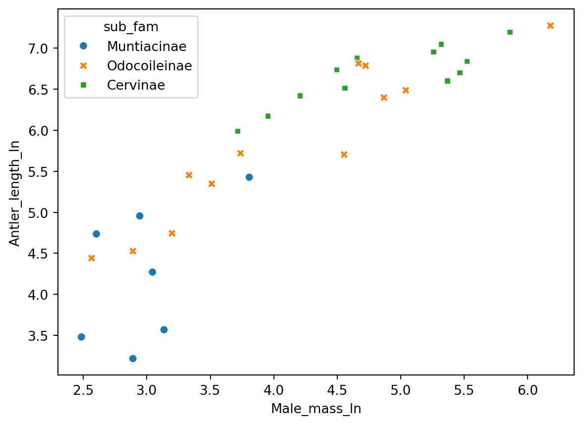
From the log-log plot, it seems that particularly the sub-family Muntiacinae appears to deviate from the linear pattern in the entire sample.
Filter antlers and only run the linear regression on a combined sample of the sub-families Odocoileinae (“New World Deer”) and Cervinae (“Old World Deer”). Check whether the expected relation between body mass and antler length holds when not considering Muntiacinae by applying the necessary parts of the above procedure to the filtered data.
antlers_fltr = antlers[antlers["sub_fam"] != "Muntiacinae"]# run regression on the filtered data
model = ols("Antler_length_ln ~ Male_mass_ln", data=antlers_fltr)
model_fit = model.fit()
model_fit.summary2()
# confidence interval
model_pred = model_fit.get_prediction()
# get prediction summery in a data frame
pred_summary = model_pred.summary_frame(alpha=0.05)
# make scatterplot including regression and confidence bands
intercept = model_fit.params.iloc[0]
slope = model_fit.params.iloc[1]
rsquared = model_fit.rsquared
p_value = model_fit.pvalues.iloc[1]
label = f'y = {intercept:.2f} + {slope:.2f}x\np = {p_value:0.2E}\nR2 = {rsquared:0.2f}'
fig, ax = plt.subplots()
ax.set_ylim(2.6,9.4)
ax.set_ylabel('ln Antler length [mm]')
ax.set_xlabel('ln Body mass [kg]')
plt.annotate(label, xy=(0.97, 0.03), xycoords='axes fraction',
fontsize=10, backgroundcolor='white',
horizontalalignment='right', verticalalignment="bottom")
ax.fill_between(antlers_fltr["Male_mass_ln"], pred_summary['obs_ci_lower'], pred_summary['obs_ci_upper'],
color='gray', alpha=0.25, edgecolor=None)
ax.fill_between(antlers_fltr["Male_mass_ln"], pred_summary['mean_ci_lower'], pred_summary['mean_ci_upper'],
color='gray', alpha=0.4, edgecolor=None)
ax.plot(antlers_fltr["Male_mass_ln"], model_fit.fittedvalues, '-', color='r', alpha=0.5)
ax.plot(antlers_fltr.Male_mass_ln, antlers_fltr.Antler_length_ln, '.', color='k')
# have a look at residual plot
fig, ax = plt.subplots()
ax.axhline(y=0.0, color='black', linestyle='--', linewidth=1)
ax.plot(antlers_fltr.Male_mass_ln, model_fit.resid, '.')
ax.set_xlabel('x')
ax.set_ylabel(r'$y-\hat{y}$')
ax.set_ylim(-0.8,0.8)
# perform breusch pagan test
if sm.stats.diagnostic.het_breuschpagan(model_fit.resid, model.exog)[1] > 0.05:
print("The residuals are homoscedasctic")
else:
print("The residuals are not homoscedasctic")The residuals are homoscedasctic
# perform shapiro-wilk test
if stats.shapiro(model_fit.resid)[1] > 0.05:
print("The residuals are normally distributed")
else:
print("The residuals are not normally distributed")The residuals are normally distributed
- Has the model improved?
- Are the assumptions for linear regression met in this case?
- The model has improved. Although the p value is slightly lower, it is still highly significant and \(R^2\) is slightly higher.
- Linearity seems much better, although there is still a slight parabola visible in the residual plot. The residuals are normally distributed and homoscedastic. Using linear regression is likely valid in this case.
Perform the procedure once more, but now separately for both subspecies of Odocoileinae and Cervinae.
# filter data
antlers_o = antlers[antlers["sub_fam"] == "Odocoileinae"]
antlers_c = antlers[antlers["sub_fam"] == "Cervinae"]
# run regression on both subsets
model_o = ols("Antler_length_ln ~ Male_mass_ln", data=antlers_o)
model_c = ols("Antler_length_ln ~ Male_mass_ln", data=antlers_c)
model_o_fit = model_o.fit()
model_c_fit = model_c.fit()# plot both species in one plot including regression lines
sns.scatterplot(
x="Male_mass_ln",
y="Antler_length_ln",
data=antlers_fltr,
hue="sub_fam",
style="sub_fam")
plt.plot(model_o.exog[:,1], model_o_fit.fittedvalues, '-', color='blue', alpha=0.5)
plt.plot(model_c.exog[:,1], model_c_fit.fittedvalues, '-', color='orange', alpha=0.5)
plt.show()
# have a look at residual plots of Odocoileinae
fig, ax = plt.subplots()
ax.set_xlabel('x')
ax.set_ylabel(r'$y-\hat{y}$')
ax.set_ylim(-0.8,0.8)
ax.axhline(y=0.0, color='black', linestyle='--', linewidth=1)
ax.plot(antlers_o.Male_mass_ln, model_o_fit.resid, '.')
# have a look at residual plots of Cervinae
fig, ax = plt.subplots()
ax.set_xlabel('x')
ax.set_ylabel(r'$y-\hat{y}$')
ax.set_ylim(-0.8,0.8)
ax.axhline(y=0.0, color='black', linestyle='--', linewidth=1)
ax.plot(antlers_c.Male_mass_ln, model_c_fit.resid, '.')
# perform breusch pagan tests
if sm.stats.diagnostic.het_breuschpagan(model_o_fit.resid, model_o.exog)[1] > 0.05:
print("The residuals are homoscedasctic")
else:
print("The residuals are not homoscedasctic")The residuals are homoscedasctic
if sm.stats.diagnostic.het_breuschpagan(model_c_fit.resid, model_c.exog)[1] > 0.05:
print("The residuals are homoscedasctic")
else:
print("The residuals are not homoscedasctic")The residuals are homoscedasctic
# perform shapiro-wilk test
if stats.shapiro(model_o_fit.resid)[1] > 0.05:
print("The residuals are normally distributed")
else:
print("The residuals are not normally distributed")The residuals are normally distributed
if stats.shapiro(model_c_fit.resid)[1] > 0.05:
print("The residuals are normally distributed")
else:
print("The residuals are not normally distributed")The residuals are normally distributed
Are the assumptions for linear regression met in both these cases?
For both models linearity, normality and homoscedasticity are OK. Using Linear regression is valid.
An interesting scientific question could be whether the relations between body mass and antler length differ significantly between different the sub families. In statistics, when the relations between two (or more) variables depend on another variable, it is called an interaction effect.
In this example, one could say: does antler length increase by a certain amount (i.e. slope of interaction effect) more per body mass unit for Odocoileinae than Cervinae? To test this hypothesis, we need to add the relevant interaction term to the model. In this case, we’ll include the interaction term Male_mass_ln * Sub-family (for more details on interaction formulations see 12.2.4 of Haslwanter, 2022).
model_comp = ols("Antler_length_ln ~ Male_mass_ln * sub_fam", data=antlers_fltr)
model_comp_fit = model_comp.fit()
print(model_comp_fit.summary2())The p-value for slope of the interaction term (the term that includes both the predictor and the group variable) indicates whether the two groups are statistically different. If the p-value is less than your predefined \(\alpha\), you can reject the null hypothesis that the slopes are equal, i.e. the slopes are significantly different.
Results: Ordinary least squares
====================================================================================
Model: OLS Adj. R-squared: 0.890
Dependent Variable: Antler_length_ln AIC: 9.6733
Date: 2026-03-06 15:57 BIC: 14.3855
No. Observations: 24 Log-Likelihood: -0.83663
Df Model: 3 F-statistic: 63.13
Df Residuals: 20 Prob (F-statistic): 2.23e-10
R-squared: 0.904 Scale: 0.075333
------------------------------------------------------------------------------------
Coef. Std.Err. t P>|t| [0.025 0.975]
------------------------------------------------------------------------------------
Intercept 4.5591 0.5875 7.7602 0.0000 3.3336 5.7847
sub_fam[T.Odocoileinae] -2.2072 0.6736 -3.2767 0.0038 -3.6124 -0.8021
Male_mass_ln 0.4344 0.1197 3.6294 0.0017 0.1847 0.6841
Male_mass_ln:sub_fam[T.Odocoileinae] 0.4073 0.1428 2.8518 0.0099 0.1094 0.7052
------------------------------------------------------------------------------------
Omnibus: 0.546 Durbin-Watson: 1.621
Prob(Omnibus): 0.761 Jarque-Bera (JB): 0.639
Skew: 0.280 Prob(JB): 0.726
Kurtosis: 2.430 Condition No.: 82
====================================================================================
Notes:
[1] Standard Errors assume that the covariance matrix of the errors is correctly
specified.
Do the two sub families that you’ve tested have a different allometric relation between body mass and antler length?
The p-value for the slope of the interaction term is 0.0099, which is below an \(\alpha\) level of 0.05 and 0.01, indicating that \(H_0\) is rejected. The allometric relations between body mass and antler length between the two sub-families are significantly different from each other.
# Final plot with non-transformed curves and allomatric relation
fig, ax = plt.subplots()
x_val = np.linspace(0, np.max(antlers.Male_body_mass), 100)
y_fit_o = np.exp(model_o_fit.params.iloc[0]) * x_val ** model_o_fit.params.iloc[1]
y_fit_c = np.exp(model_c_fit.params.iloc[0]) * x_val ** model_c_fit.params.iloc[1]
ax.set_ylabel('Antler length [mm]')
ax.set_xlabel('Body mass [kg]')
label = f'y = {np.exp(model_o_fit.params.iloc[0]):.2f}*x^{model_o_fit.params.iloc[1]:.2f}\ny = {np.exp(model_c_fit.params.iloc[0]):.2f}*x^{model_c_fit.params.iloc[1]:.2f}'
plt.annotate(label, xy=(0.97, 0.03), xycoords='axes fraction',
fontsize=10, backgroundcolor='white',
horizontalalignment='right', verticalalignment="bottom")
ax.plot(x_val, y_fit_o, '-', color='blue', alpha=0.5)
ax.plot(x_val, y_fit_c, '-', color='red', alpha=0.5)
ax.plot(antlers_o.Male_body_mass, antlers_o.Antler_length, '.', color='blue')
ax.plot(antlers_c.Male_body_mass, antlers_c.Antler_length, '.', color='red')
References
- Haslwanter, T., 2022. An Introduction to Statistics with Python: With Applications in the Life Sciences, Second. ed, Statistics and Computing. Springer International Publishing, Cham. https://doi.org/10.1007/978-3-030-97371-1
- Plard, F., Bonenfant, C., Gaillard, J.-M., 2011. Revisiting the allometry of antlers among deer species: male–male sexual competition as a driver. Oikos 120, 601–606. https://doi.org/10.1111/j.1600-0706.2010.18934.x
- Tsuboi, M., Kopperud, B.T., Matschiner, M., Grabowski, M., Syrowatka, C., Pélabon, C., Hansen, T.F., 2024. Antler Allometry, the Irish Elk and Gould Revisited. Evol Biol 51, 149–165. https://doi.org/10.1007/s11692-023-09624-1